Non-Dimensional Outputs#
Note
With User Variables, manual dimensionalization is rarely needed — simply request the desired unit system and the conversion is automatic. The formulas below describe the underlying logic.
All solver outputs are non-dimensional. To recover physical (SI) values, multiply by the appropriate reference quantity from the Reference Quantities Table.
Property |
Ref. value for nondim. |
Examples of non-dimensional outputs in Flow360 |
|---|---|---|
Length |
\(L_\text{gridUnit}\) |
|
Density |
\(\rho_\infty\) |
|
Velocity |
\(U_\text{scale}\) (reference velocity scaling) |
|
Pressure |
\(\rho_\infty U_\text{scale}^2\) where \(U_\text{scale}\) is the reference velocity scaling |
|
Temperature |
\(T_\infty\) |
|
Heat Flux |
\(\rho_\infty U_\text{scale}^3\) where \(U_\text{scale}\) is the reference velocity scaling |
|
BET, Actuator Disk and Porous Media Force |
\(\rho_\infty U_\text{scale}^2 L_\text{gridUnit}^2\) where \(U_\text{scale}\) is the reference velocity scaling |
force in BET output |
BET, Actuator Disk and Porous Media Moment |
\(\rho_\infty U_\text{scale}^2 L_\text{gridUnit}^3\) where \(U_\text{scale}\) is the reference velocity scaling |
moment in BET output |
Note
Many output variables use the reference velocity scaling \(U_\text{scale}\) (not \(U_\text{ref}\)). In the examples below we assume \(U_\text{scale}\) has been computed as shown in the Introduction.
Visualization Field Conversions#
Flow360 exports ParaView (.pvtu) and Tecplot (.szplt) files. All exported fields are non-dimensional. The subsections below show how to recover dimensional values.
Accessing case results.#
Velocity#
Reference value: \(U_\text{scale}\).
If velocityX = 0.6 and \(U_\text{scale} = 340\;\text{m/s}\), then \(v_x = 0.6 \times 340 = 204\;\text{m/s}\).
Pressure#
Reference value: \(\rho_\infty\,U_\text{scale}^2\).
If p = 0.65, \(\rho_\infty = 1.225\;\text{kg/m}^3\), and \(U_\text{scale} = 340\;\text{m/s}\):
Node Force Per Unit Area#
nodeForcesPerUnitArea is the total (pressure + friction) force at a node divided by the surface area attributed to that node. Integrating over the whole surface yields the total force. The reference value is the same as for pressure: \(\rho_\infty\,U_\text{scale}^2\).
Temperature#
Reference value: \(T_\infty\). Multiply the non-dimensional temperature by the freestream temperature to obtain Kelvin.
Surface Coefficient Definitions#
The following coefficients appear in both visualization files and CSV files. They all use the reference velocity \(U_\text{ref}\) (accessed via case.params.reference_velocity), which is different from \(U_\text{scale}\).
Tip
Flow360’s unit system carries SI units through arithmetic, so you can convert any coefficient to physical units in one step. For example, once q_ref and A_ref are retrieved from the API:
tau_wall = (Cf * q_ref).to('Pa')           # wall shear stress
p_dim    = (Cp * q_ref + p_inf).to('Pa')   # static pressure
We define the dynamic pressure for coefficients as:
Skin Friction Coefficient#
The skin friction coefficient vector \(\mathbf{C_f}\) and its magnitude \(C_f\):
To recover the dimensional wall shear stress:
Pressure Coefficient#
To recover the dimensional static pressure:
Total Pressure Coefficient#
To recover the dimensional total pressure:
The total pressure coefficient can also be computed from the primitive variables as described in equations 26 and 29 of this paper:
where \(\gamma = 1.4\) for standard air.
Note
Ensure Mach and primitiveVars are included in your volume output configuration.
CSV File Outputs#
Actuator Disk#
The file actuatorDisk_output_v2.csv reports power, force, and moment for each disk. The power column contains a coefficient:
To obtain dimensional power:
actuator_disk_output = case.results.actuator_disks.averages
density = case.params.operating_condition.thermal_state.density
L_grid  = project.length_unit

C_p   = actuator_disk_output['Disk0_Power']
power = C_p * density * U_scale**3 * L_grid**2      # W
Attention
Actuator Disk forces and moments use \(U_\text{scale}\), not \(U_\text{ref}\). See Converting to Physical Units for the general conversion formulas.
BET Loading#
The file bet_forces_v2.csv contains:
Integrated forces and moments per disk (
Disk0_Force_x,Disk0_Moment_x, …). These are non-dimensional raw values:(11)#\[\text{Force}^* = \frac{F\;[\text{N}]}{\rho_\infty\,U_\text{scale}^2\,L_\text{gridUnit}^2}\](12)#\[\text{Moment}^* = \frac{M\;[\text{N·m}]}{\rho_\infty\,U_\text{scale}^2\,L_\text{gridUnit}^3}\]Note
These values represent forces/moments on the solid. Forces on the fluid are the negative of the above.
Note
Equations Eq.(11) and Eq.(12) also apply to Porous Media outputs in
porous_media_output_v2.csv.Attention
BET forces and moments use \(U_\text{scale}\), not \(U_\text{ref}\). The x, y, z components are in the global inertial frame defined by the mesh.
Sectional thrust \(C_t\) and torque \(C_q\) per blade at each radial station (
Disk0_Blade0_R0_ThrustCoeff, …).(13)#\[C_t(r) = \frac{\text{Thrust/span}\;[\text{N/m}]}{\tfrac{1}{2}\,\rho_\infty\,(\Omega r)^2\,\text{chord}_\text{ref}} \cdot \frac{r}{R}\](14)#\[C_q(r) = \frac{\text{Torque/span}\;[\text{N}]}{\tfrac{1}{2}\,\rho_\infty\,(\Omega r)^2\,\text{chord}_\text{ref}\,R} \cdot \frac{r}{R}\]Here \(r\) is the dimensional distance from the rotation axis, \(\text{chord}_\text{ref}\) the dimensional reference chord, and \(R\) the rotor radius.
Note
\(C_t\) and \(C_q\) are sectional loadings: \(C_t(r) = \text{d}C_T/\text{d}(r/R)\) and \(C_q(r) = \text{d}C_Q/\text{d}(r/R)\).
Important
All right-hand-side quantities in Eq.(11)–Eq.(14) are dimensional. The non-dimensional radius in the CSV must first be converted: \(r\) =
Disk0_Blade0_R0_Radius\(\times\, L_\text{gridUnit}\).Warning
For steady-state BET Disk simulations, \(C_t\) and \(C_q\) are written only for
Blade0; all other blades report zeros because the loading is identical. For unsteady BET Line simulations each blade has distinct values.
Python example — dimensional force, moment, and sectional loading:
bet_forces = case.results.bet_forces.averages
density    = case.params.operating_condition.thermal_state.density
L_grid     = project.length_unit

# --- Integrated force & moment (Disk 0) ---
force_x  = bet_forces["Disk0_Force_x"]  * density * U_scale**2 * L_grid**2     # N
moment_x = bet_forces["Disk0_Moment_x"] * density * U_scale**2 * L_grid**3     # N·m

# --- Sectional loading (Disk 0, Blade 0, radial station 1) ---
bet_model  = case.params.models[4]   # index of the BETDisk model
chord_ref  = bet_model.chord_ref
omega      = bet_model.omega
R          = bet_model.entities.stored_entities[0].outer_radius

r1    = bet_forces["Disk0_Blade0_R1_Radius"]
Ct_r1 = bet_forces["Disk0_Blade0_R1_ThrustCoeff"]
Cq_r1 = bet_forces["Disk0_Blade0_R1_TorqueCoeff"]

thrust_r1 = Ct_r1 * 0.5 * density * omega**2 * r1 * L_grid * R * chord_ref     # N/m
torque_r1 = Cq_r1 * 0.5 * density * omega**2 * r1 * L_grid * R**2 * chord_ref  # N
Aeroacoustic Output#
The file total_acoustics_v3.csv reports the non-dimensional acoustic pressure signal at each observer location. If AeroacousticOutput.write_per_surface_output is True, per-surface files surface_<name>_acoustics_v3.csv are also written.
Columns: time, physical_step, observer_0_pressure, observer_0_thickness, observer_0_loading, … for N+1 observers.
Note
The observation time may fall outside the simulation time range because the acoustic signal takes a finite propagation time from the surface to each observer. Early and late time entries are zero-padded.
Heat Transfer#
The file surface_heat_transfer_v2.csv contains surface-integrated heat flux in non-dimensional form.
To recover the dimensional heat transfer rate, multiply by \(\rho_\infty\,U_\text{scale}^3\,L_\text{gridUnit}^2\):
surface_ht = case.results.surface_heat_transfer.averages
density    = case.params.operating_condition.thermal_state.density
L_grid     = project.length_unit

q_nd = surface_ht["fluid/Interface_solid_HeatTransferRate"]
q    = q_nd * density * U_scale**3 * L_grid**2   # W
Visualization Tips#
The sections below are not about conversion formulas but about using specific output fields effectively.
Skin Friction — Detecting Separation#
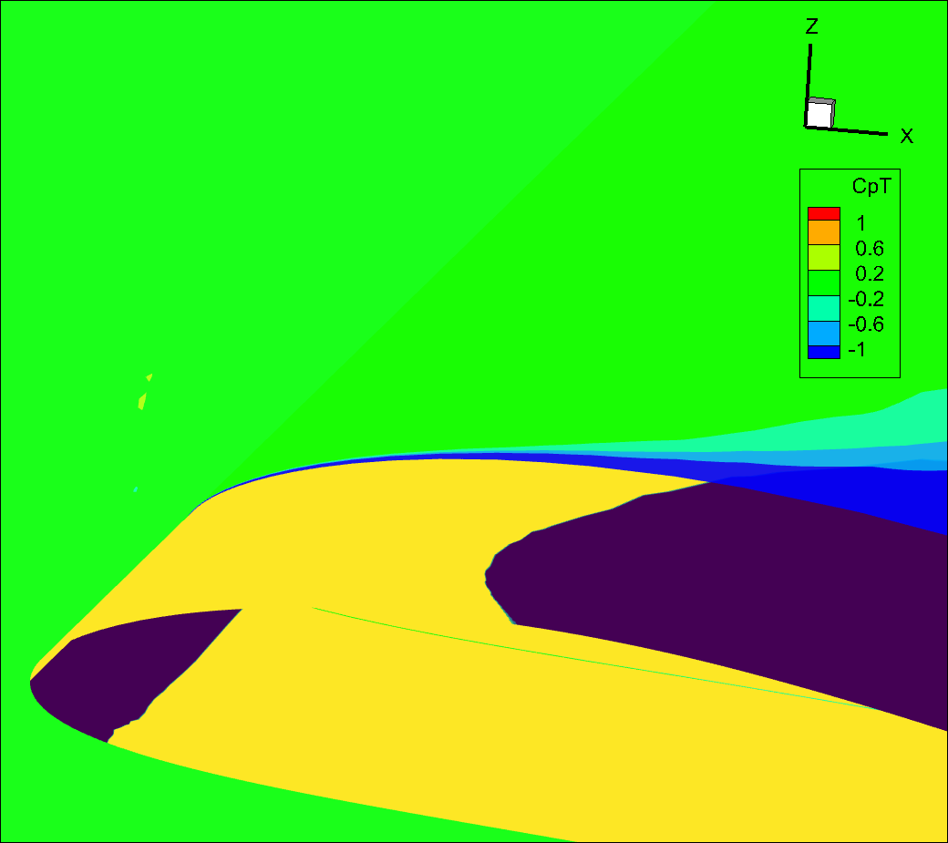
The CfVec vector is useful for locating boundary-layer separation. Fully attached flow follows the surface along the streamwise direction; separated flow produces local recirculation with reversed skin friction.
For flow predominantly in the x-direction, regions of negative CfVecX indicate separation. Visualizing with a three-level scale (e.g. −1e-6, 0, 1e-6) highlights separated vs. attached regions:
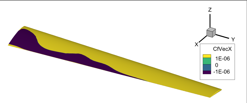
x-component of skin friction showing attached (yellow) and separated (purple) flow at high angle of attack.#
Surface streamlines can also reveal recirculation. Since wall velocity is zero on a NoSlipWall, use CfVec{X,Y,Z} as the integration variable instead of velocity:
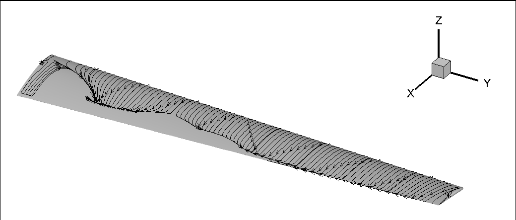
Surface streamlines showing recirculation regions.#
Total Pressure — Visualizing Separation and Boundary Layers#
\(C_{p_t}\) reveals separation regions in volume slices and is effective for visualizing the boundary layer:
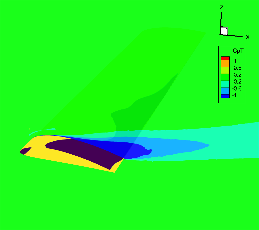
Total pressure coefficient on a slice through a partially stalled wing.#
Zoomed view showing the developing boundary layer (blue) near the leading edge.#
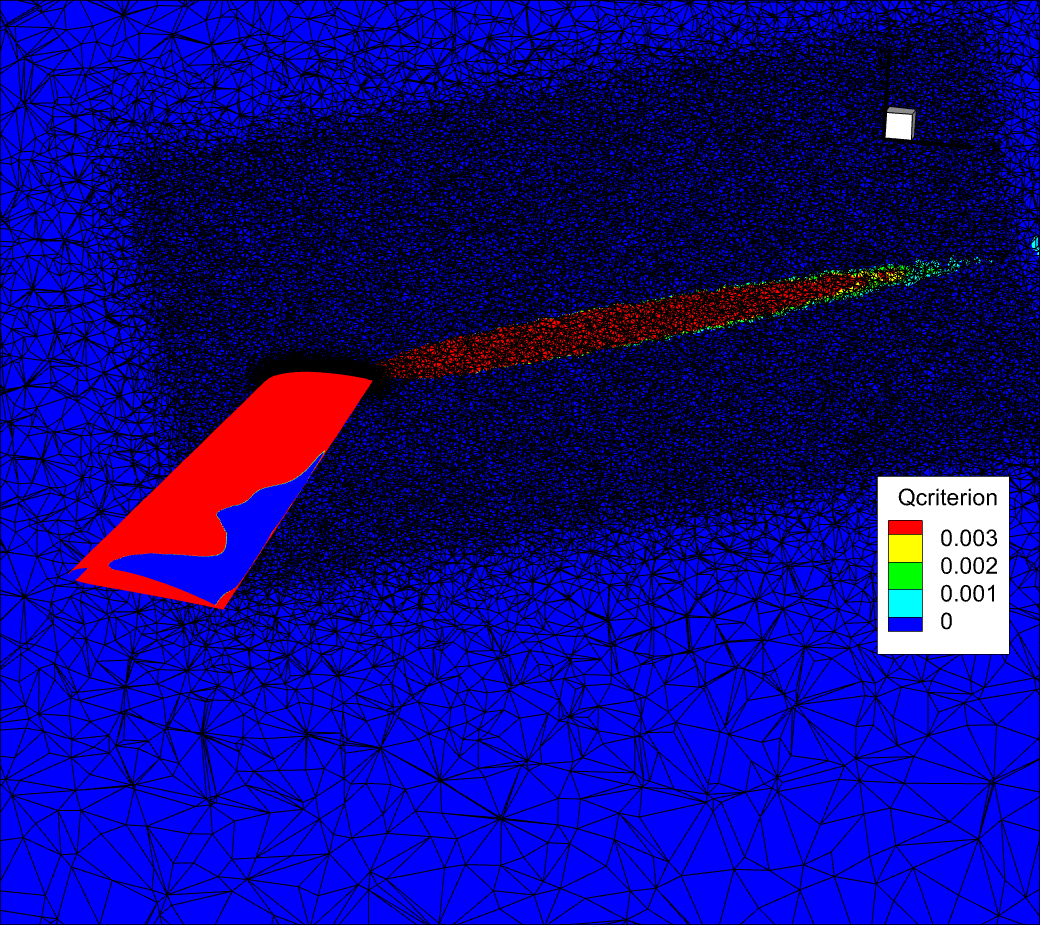
Q-Criterion — Visualizing Vortices#
The qcriterion field identifies vortices via isosurfaces. Recommended isosurface values:
Aircraft: \(\text{Ma}^2 / \text{span}^2\)
Rotors: \(\text{Ma}_\text{tip}^2 / D^2\)
Larger values show only strong vortices; smaller values reveal weaker structures.
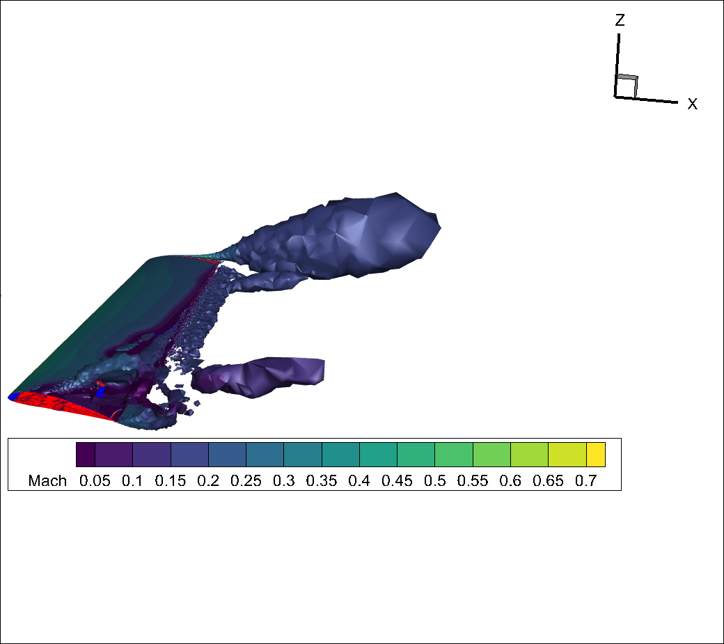
qcriterion isosurface showing tip vortex and vortices from the separation region.#
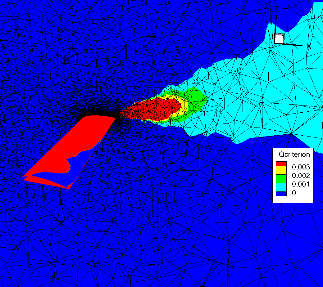
Volume mesh coarsening away from the wing causes rapid vortex dissipation.#
After refining the far-field mesh:
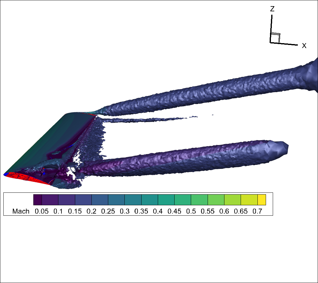
Smoother isosurface with improved vortex resolution on a refined mesh.#
Refined volume mesh reduces numerical dissipation.#
For more Q-criterion visualizations: