Download notebook (.ipynb)

Download script (.py)

Unsteady DDES HLPW4

Accurate predictions at large angles of attack (AOA) are crucial for aircraft CFD simulations, particularly for estimating stall speed and post-stall behavior. However, since RANS models rely on a time-averaged formulation, they inherently filter out flow unsteadiness and cannot capture phenomena such as vortex shedding, transient reattachment, and fluctuating separation bubbles. As a result, RANS often predicts flow separation either too early or too late, and the size and location of the recirculation region are typically inaccurate.

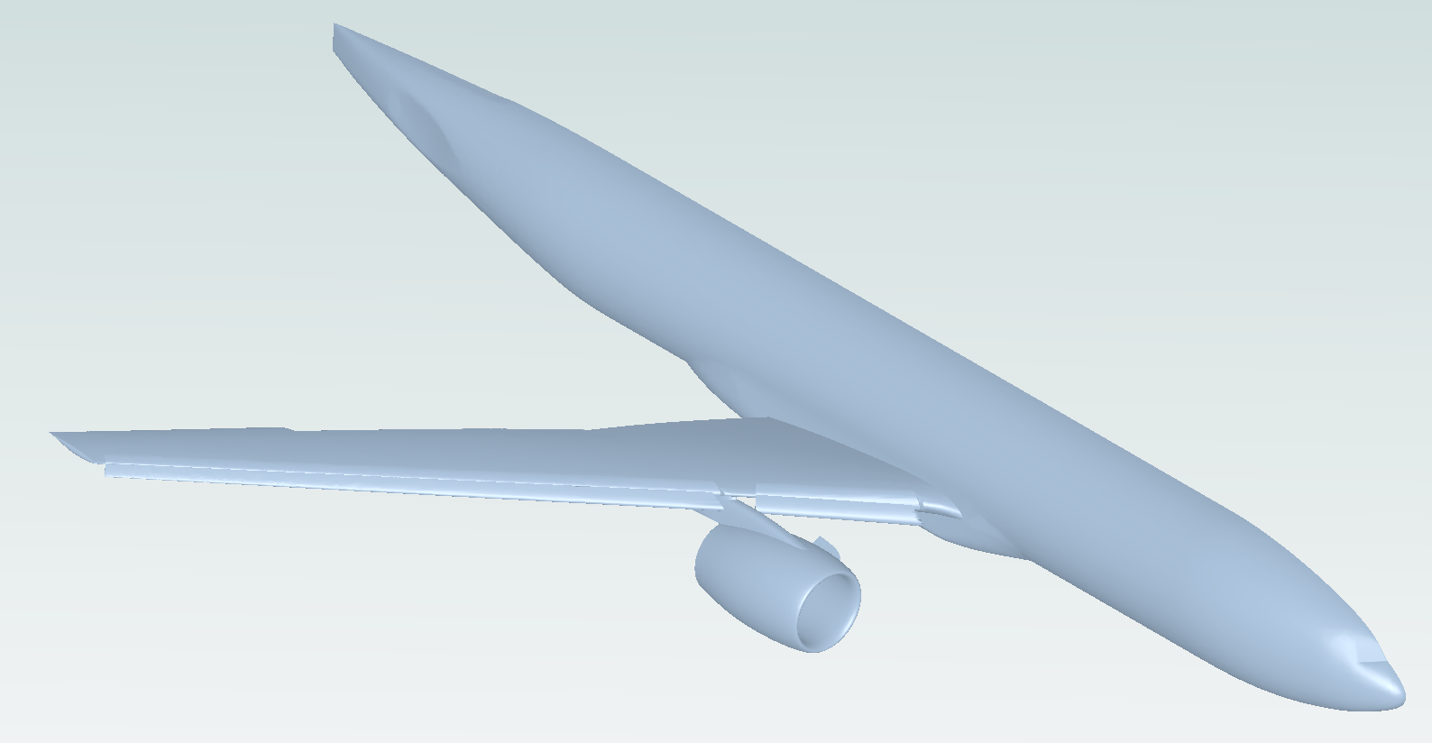
In this example, the HiLiftPW-4 (HLPW4) case is used to demonstrate the Flow360 workflow for performing an unsteady simulation using DDES to model high-AOA conditions where flow separation is expected. The computational mesh can be downloaded from the website: https://hiliftpw-committee.github.io/HLPW/index-workshop4.html. Specifically, the mesh file used is HLPW-4_CRM-HL_40-37_Nominal_v1a_Unstr-Hex-Prism-Pyr-Tet_Level-D (2.3.D). In this example, the ugrid file are used, although the CGNS format of the mesh is also supported for Flow360.

1. Create Project from Volume Mesh

In this example, the workflow begins with a volume mesh. When the mesh is uploaded to the cloud, a project is automatically created, and a unique project ID will be assigned. Typically, the mesh file to be uploaded is stored on the local machine, so user needs to specify the file path and name. At the same time, the user can select the unit system used to build the mesh and define the project name.

import flow360 as fl

project = fl.Project.from_cloud(project_id="prj-98fb1425-2354-42c2-81f8-75f890ccfe29")
mesh_object = project.volume_mesh

2. Define time steps

In this step we define the unsteady time-stepping settings for the DDES simulation using fl.Unsteady. The code below specifies the number of physical steps, the physical time-step size, the maximum number of pseudo-steps per physical step, and the CFL strategy which in this case we use adaptive CFL.

time_stepping = fl.Unsteady(
    max_pseudo_steps=35,
    steps=600,
    step_size=0.001 * fl.u.s,
    CFL=fl.AdaptiveCFL(),  # Optionally switch to CFL=fl.RampCFL()
)

3. DDES setting

The DDES (Delayed Detached Eddy Simulation) option enables a hybrid turbulence modeling approach suitable only for unsteady flow simulations. It is recommended for cases involving complex flow physics, such as significant separation regions or bluff body flows, as it provides higher solution fidelity than pure RANS models. To use DDES, define the turbulence model as below:

turbulence_model_solver = fl.SpalartAllmaras(
    absolute_tolerance=1e-8,
    relative_tolerance=1e-2,
    linear_solver=fl.LinearSolver(max_iterations=25),
    hybrid_model=fl.DetachedEddySimulation(shielding_function="DDES"),
    rotation_correction=True,
    equation_evaluation_frequency=1,
)

4. Outputs

A dedicated output metric has been developed for DDES simulations, available as either SpalartAllmaras_hybridModel or kOmegaSST_hybridModel, depending on the turbulence model selected by the user. This metric provides five key DDES-related variables:

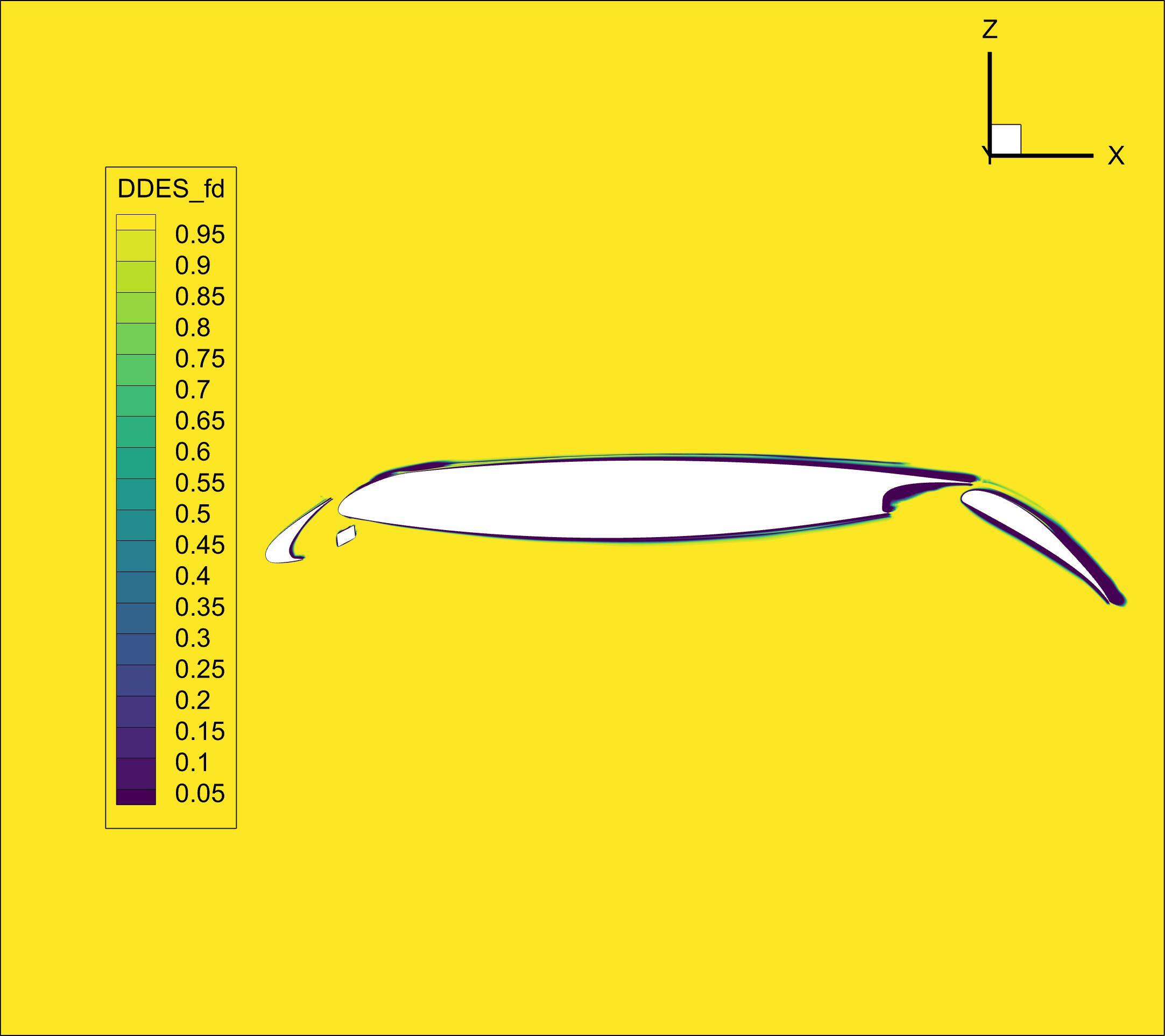
1. f_d – The shielding function that delineates the RANS and LES regions. When f_d = 0, the RANS model is fully applied; when f_d = 1, the LES model is used. Intermediate values represent a smooth transition between the two regimes.

2. r_d – A modified ratio of the modeled length scale to the wall distance, from which f_d is derived.

3. DDES_lengthRANS – The wall distance from the computational cell to the nearest solid boundary.

4. DDES_lengthScale - The characteristic DES length scale

   (5.3.10)\[\tilde{d} \equiv d - f_d \max(0, d - C_{DES}*\Delta)\]

5. DDES_lengthLES – The characteristic LES length scale,

   (5.3.11)\[C_{DES}*\Delta\]

Among these variables, f_d is the most significant, as it enables users to identify and visualize the regions dominated by RANS and DES behavior within the computational domain.

volume_outputs = fl.VolumeOutput(
    name="volume_outputs",
    output_fields=["SpalartAllmaras_hybridModel"],
    output_format="tecplot",
)

Additionally, for unsteady simulations, users may be interested in the time history of a flow field property. The following example shows a typical case where Q-criterion isosurfaces are output at a frequency of 20, with Mach number as the output field.

iso_surface = fl.IsosurfaceOutput(
    isosurfaces=[
        fl.Isosurface(
            name="Isosurface_Q_cri",
            iso_value=1e-6,
            field="qcriterion",
        ),
    ],
    output_format="tecplot",
    output_fields=["Mach"],
    frequency=20,
    frequency_offset=0,
)

5. Define Simulation Parameters

For Flow360 simulations, the operating conditions, boundary conditions (which depend on the surface names of the mesh), reference geometry, and solver settings can be defined in the same way as in other examples. For brevity, user can refer to those cases for detailed descriptions. The settings for this example are provided below, including the DDES configuration to illustrate the complete model setup.

with fl.SI_unit_system:
    params = fl.SimulationParams(
        time_stepping=time_stepping,
        operating_condition=fl.AerospaceCondition.from_mach(
            mach=0.2,
            alpha=17.05 * fl.u.deg,
            thermal_state=fl.ThermalState(
                temperature=289.44 * fl.u.K,
                density=0.002063 * fl.u.kg / fl.u.m**3,
                material=fl.Air(),
            ),
            reference_mach=0.2,
        ),
        reference_geometry=fl.ReferenceGeometry(),
        models=[
            fl.Wall(
                surfaces=[
                    mesh_object["1"],
                    mesh_object["3"],
                    mesh_object["4"],
                    mesh_object["5"],
                    mesh_object["6"],
                    mesh_object["7"],
                    mesh_object["8"],
                    mesh_object["9"],
                    mesh_object["11"],
                ],
            ),
            fl.Freestream(surfaces=mesh_object["2"]),
            fl.SlipWall(surfaces=mesh_object["10"]),
            fl.Fluid(
                navier_stokes_solver=fl.NavierStokesSolver(
                    absolute_tolerance=1e-10,
                    relative_tolerance=1e-2,
                    linear_solver=fl.LinearSolver(max_iterations=35),
                    kappa_MUSCL=-1,
                    numerical_dissipation_factor=1.0,
                ),
                turbulence_model_solver=turbulence_model_solver,
            ),
        ],
        outputs=[volume_outputs, iso_surface],
    )

[11:28:58] INFO: using: SI unit system for unit inference.

6. Run case

To run a case we need the previously defined params object to run the case in the project.

case = project.run_case(params=params, name="DDES HLPW4 from Python")

           INFO: using: SI unit system for unit inference.

[11:29:00] INFO: Successfully submitted:
                   type        = Case
                   name        = DDES HLPW4 from Python
                   id          = case-ff225dfb-3aac-4e4d-bf53-bf8b2ed09181
                   status      = pending
                   project id  = prj-98fb1425-2354-42c2-81f8-75f890ccfe29