Adjoint optimization of a photonic crystal#
In this notebook, we will use inverse design to optimize coupling from a silicon waveguide to a photonic crystal slab.
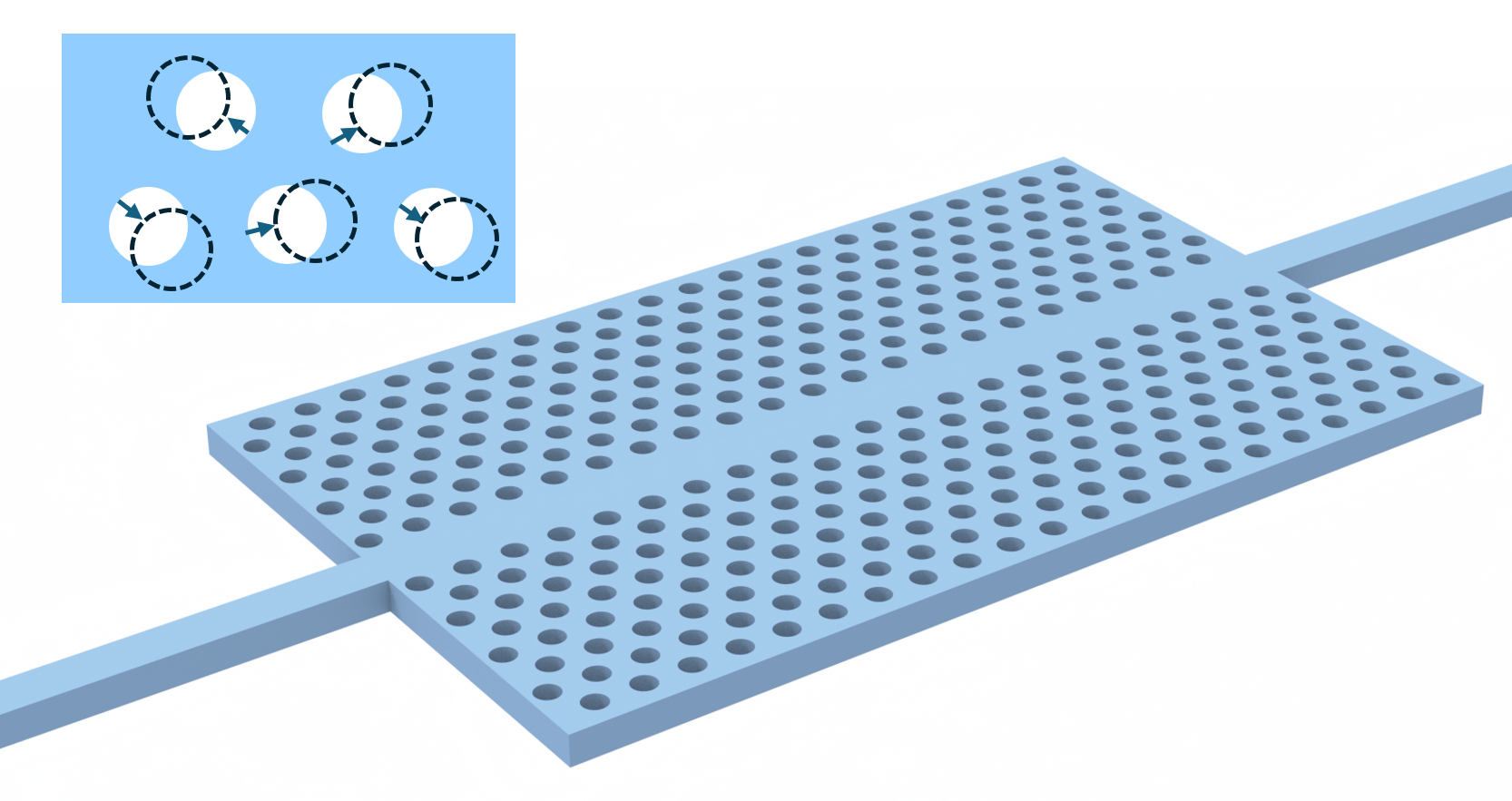
We’ll first set up a very simple photonic crystal in a silicon slab.
Then, we’ll maximize the transmitted flux through the crystal at a frequency just above the bandgap.
Our degrees of freedom will be the center of the holes cut in the photonic crystal, but modifying this example, one can easily adjust the radius of each hole as well as an extra design parameter.
If you are unfamiliar with inverse design, we also recommend our intro to inverse design tutorials and our primer on automatic differentiation with tidy3d.
[1]:
import autograd

# we'll use autograd for automatic differentiation, so derivative-traced numpy operations will use autograd.numpy
import autograd.numpy as anp
import matplotlib.pyplot as plt
import numpy as np
import tidy3d as td
import tidy3d.web as web
Setup#
First, we will set up some of our global parameters for the study.
The structure will consist of a rectangular lattice of air holes in a silicon slab.
[2]:
nm = 1e-3

wvl0 = 1550 * nm
a = 400 * nm

num_freqs = 151

wvl_min, wvl_max = (1400 * nm, 1700 * nm)
freq_min = td.C_0 / wvl_max
freq_max = td.C_0 / wvl_min

freqs = np.linspace(freq_min, freq_max, num_freqs)
freq0 = td.C_0 / wvl0

fwidth = freq0 / 10
run_time = 300 / fwidth

sqrt3_div2 = np.sqrt(3) / 2.0
[3]:
# silicon material (for slab)
n_si = 3.48
si = td.Medium(permittivity=n_si**2)
air = td.Medium()
[4]:
# radius of holes
r0 = 90 * nm

# when we optimize, the radius will vary between these two values
# for now we just constrain all radius to r0, but change these values to add more degrees of freedom
r_range = rmin, rmax = (r0, r0)
rmid = r0

# how much centers can move from the center
drmax = a / 4
[5]:
# number of holes in x and y
N_rows = 15
N_cols = 19
N_cols_static = 5

# total length of the PhC region
Lx_phc = N_cols * a + a / 2
Ly_phc = N_rows * sqrt3_div2 * a + a / 2

# buffer on each side of the design region
buffer = 1.0 * wvl0

# thickness of slab
t_slab = 220 * nm

# waveguide width
w_wg = 1.3 * a
[6]:
# size of simulation
Lx = Lx_phc + 2 * buffer
Ly = Ly_phc + 2 * buffer
Lz = t_slab + 2 * buffer
[7]:
# define grid resolution
steps_per_unit_cell = 14
dx = a / steps_per_unit_cell
dy = a * sqrt3_div2 / steps_per_unit_cell

grid_spec = td.GridSpec(
    grid_x=td.UniformGrid(dl=dx),
    grid_y=td.UniformGrid(dl=dy),
    grid_z=td.AutoGrid(min_steps_per_wvl=steps_per_unit_cell),
)
[8]:
def make_holes(params) -> td.Structure:
    """Convenience function to make the phc holes given the design parameters."""

    hole_spacing_x = a
    hole_spacing_y = a * sqrt3_div2

    x_slab_length, y_slab_length = (
        hole_spacing_x * (N_cols + 0.5),
        hole_spacing_y * N_rows,
    )
    start_x, start_y = (
        -x_slab_length / 2 + hole_spacing_x / 2,
        -y_slab_length / 2 + hole_spacing_y / 2,
    )

    cylinders = []

    for i in range(0, N_cols):
        for j in range(0, N_rows):
            # depending on distance from central column, hole is either static
            i_dist = abs(i - N_cols // 2)
            if i_dist < ((N_cols_static) / 2):
                radius = rmid
                dx = dy = 0

            # or optimizable
            else:
                radius = params[0, i, j]
                dx = params[1, i, j]
                dy = params[2, i, j]

            x0 = dx + start_x + (i + (j % 2) * 0.5) * hole_spacing_x
            y0 = dy + start_y + j * hole_spacing_y
            if j != N_rows // 2:
                c = td.Cylinder(
                    axis=2,
                    radius=radius,
                    center=(x0, y0, 0),
                    length=td.inf,
                )
                cylinders.append(c)

    # use GeometryGroup since all same medium, for performance
    structure = td.Structure(
        geometry=td.GeometryGroup(geometries=cylinders),
        medium=air,
        background_medium=si,  # note: we need this for correct gradients when embedded in slab
    )

    return structure
[9]:
source = td.ModeSource(
    center=(-Lx / 2 + wvl0 / 10, 0, 0),
    size=(0, Ly_phc / 2.0, td.inf),
    source_time=td.GaussianPulse(freq0=freq0, fwidth=fwidth),
    direction="+",
)
[10]:
# these monitors are just for plotting the broadband flux response, not optimizing
# FluxMonitor is not supported in autograd

slab = td.Structure(
    geometry=td.Box(
        center=(0, 0, 0),
        size=(Lx_phc, Ly_phc, t_slab),
    ),
    medium=si,
)

waveguide = td.Structure(
    geometry=td.Box(
        center=(0, 0, 0),
        size=(td.inf, w_wg, t_slab),
    ),
    medium=si,
)


mnt_flux = td.FluxMonitor(
    center=(-source.center[0], 0, 0),
    size=(0, td.inf, td.inf),
    freqs=freqs,
    name="flux",
)

# this monitor is for visualizing field patterns only
mnt_field = td.FieldMonitor(
    center=(0, 0, 0),
    size=(td.inf, td.inf, 0),
    freqs=[freq0],
    name="field",
)

# These monitors are used for the optimization
# FieldMonitor.flux is used because FluxMonitor not supported in autograd

mnt_field_flux = td.FieldMonitor(
    center=(+Lx_phc / 2 - a, 0, 0),
    size=(0, td.inf, td.inf),
    freqs=[freq0],
    name="flux",
)
[11]:
def make_sim(params, optimization_mode: bool = False) -> td.Simulation:
    """Function to generate a simulation with different monitors depending on whether optimizing."""

    # create the holes
    holes = make_holes(params)

    # decide which monitors to include
    if not optimization_mode:
        monitors = [mnt_flux, mnt_field]
    else:
        monitors = [mnt_field_flux]

    return td.Simulation(
        center=[0, 0, 0],
        size=[Lx, Ly, Lz],
        grid_spec=grid_spec,
        structures=[slab, waveguide, holes],
        sources=[source],
        monitors=monitors,
        run_time=run_time,
        boundary_spec=td.BoundarySpec.pml(x=True, y=True, z=True),
        symmetry=(0, -1, 1),
    )
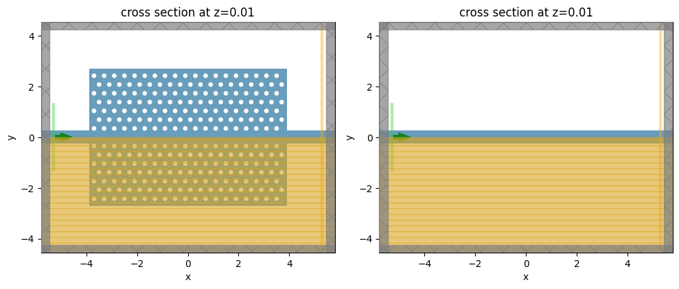
Let’s make a simulation with the starting parameters, and one with just the waveguide, for normalization.
[12]:
params0 = rmid * np.ones((3, N_cols, N_rows))
params0[1:] = 0.0

sim0 = make_sim(params0, optimization_mode=False)

sim_wg = sim0.updated_copy(structures=[waveguide])
[13]:
_, (ax1, ax2) = plt.subplots(1, 2, tight_layout=True, figsize=(10, 4))
_ = sim0.plot(z=0.01, ax=ax1)
_ = sim_wg.plot(z=0.01, ax=ax2)

plt.show()
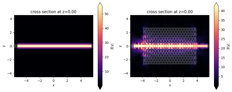
Next, we can run these two simulations to inspect the fields and compute some normalization.
[14]:
sim_data0 = web.Job(simulation=sim0, task_name="initial PhC").run()
sim_data_wg = web.Job(simulation=sim_wg, task_name="initial PhC norm").run()
11:48:23 CET Created task 'initial PhC' with resource_id
             'fdve-eae198a8-f2ea-4eb7-b104-76dede0a001e' and task_type 'FDTD'.
             View task using web UI at
             'https://tidy3d.simulation.cloud/workbench?taskId=fdve-eae198a8-f2e
             a-4eb7-b104-76dede0a001e'.
Task folder: 'default'.
11:48:33 CET Estimated FlexCredit cost: 0.252. Minimum cost depends on task
             execution details. Use 'web.real_cost(task_id)' to get the billed
             FlexCredit cost after a simulation run.
11:48:35 CET status = queued
             To cancel the simulation, use 'web.abort(task_id)' or
             'web.delete(task_id)' or abort/delete the task in the web UI.
             Terminating the Python script will not stop the job running on the
             cloud.
11:49:09 CET status = preprocess
11:49:14 CET starting up solver
running solver
11:49:55 CET early shutoff detected at 46%, exiting.
status = postprocess
11:49:56 CET status = success
11:49:58 CET View simulation result at
             'https://tidy3d.simulation.cloud/workbench?taskId=fdve-eae198a8-f2e
             a-4eb7-b104-76dede0a001e'.
11:50:02 CET Loading results from simulation_data.hdf5
             Created task 'initial PhC norm' with resource_id
             'fdve-f190bec5-eb97-45d4-b184-be15cdd72fd6' and task_type 'FDTD'.
             View task using web UI at
             'https://tidy3d.simulation.cloud/workbench?taskId=fdve-f190bec5-eb9
             7-45d4-b184-be15cdd72fd6'.
Task folder: 'default'.
11:50:15 CET Estimated FlexCredit cost: 0.252. Minimum cost depends on task
             execution details. Use 'web.real_cost(task_id)' to get the billed
             FlexCredit cost after a simulation run.
11:50:16 CET status = queued
             To cancel the simulation, use 'web.abort(task_id)' or
             'web.delete(task_id)' or abort/delete the task in the web UI.
             Terminating the Python script will not stop the job running on the
             cloud.
11:50:34 CET status = preprocess
11:50:39 CET starting up solver
running solver
11:50:41 CET early shutoff detected at 1%, exiting.
11:50:42 CET status = postprocess
status = success
11:50:44 CET View simulation result at
             'https://tidy3d.simulation.cloud/workbench?taskId=fdve-f190bec5-eb9
             7-45d4-b184-be15cdd72fd6'.
11:50:48 CET Loading results from simulation_data.hdf5
[15]:
_, (ax1, ax2) = plt.subplots(1, 2, tight_layout=True, figsize=(10, 4))
_ = sim_data_wg.plot_field("field", field_name="Ey", val="abs", ax=ax1)
_ = sim_data0.plot_field("field", field_name="Ey", val="abs", ax=ax2)

plt.show()
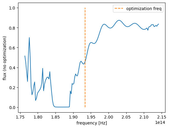
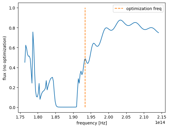
Let’s visualize the transmission. We can clearly see the bandgap, but above the bandgap, the transmission is not great. We will optimize transmitted flux at the orange line.
Note: one can also do this with
ModeMonitorand include a broadband objective.
[16]:
flux_wg = abs(sim_data_wg["flux"].flux)
flux0 = abs(sim_data0["flux"].flux) / flux_wg
flux0.plot(x="f")
plt.ylabel("flux (no optimization)")
plt.plot([freq0, freq0], [0, 1], linestyle="--", label="optimization freq")
plt.legend()
plt.show()
[17]:
flux_wg = abs(sim_data_wg["flux"].flux)
flux0 = abs(sim_data0["flux"].flux) / flux_wg
flux0.plot(x="f")
plt.ylabel("flux (no optimization)")
plt.plot([freq0, freq0], [0, 1], linestyle="--", label="optimization freq")
plt.legend()
plt.show()
[18]:
flux0_freq0 = flux_wg.interp(f=freq0).item()
print(flux0_freq0)
0.9999248769975477
The normalization flux is about 1, which is as expected as our ModeSource takes this into account.
Optimization#
Next, we will define our inverse design problem. We’ll adjust the centers and radii (if desired) to maximize flux at freq0, normalized by our straight waveguide transmission.
[19]:
def objective(params: anp.ndarray) -> float:
    """Maximize flux in -y, minimize flux in +x."""

    sim = make_sim(params, optimization_mode=True)
    sim_data = web.run(sim, task_name="phc_adjoint", verbose=False)

    flux_measure_freq0 = anp.sum(anp.abs(sim_data["flux"].flux.data))

    return flux_measure_freq0 / flux_wg.interp(f=freq0).item()
As always, we can use one line of autograd code to get a function that gives the value and gradient of our objective when passed some parameters.
[20]:
val_grad = autograd.value_and_grad(objective)
And then we can use this function in our gradient-ascent optimizer using Tidy3D’s built-in Adam helper.
We first set up the optimizer parameters.
[21]:
from autograd.tracer import getval
from tidy3d.plugins.autograd import adam, optimize

# hyperparameters
num_steps = 10
learning_rate = a / 40
# note: the step size needs to be quite low because of the direct modification of geometric parameter

# initialize adam optimizer with starting parameters
params = np.array(params0).copy()
optimizer = adam(learning_rate=learning_rate)

# store history
objective_history = []
param_history = []
data_history = []

# define lower and upper bounds for the optimization
lower_bounds = np.zeros_like(params0)
upper_bounds = np.zeros_like(params0)
lower_bounds[0] = rmin
upper_bounds[0] = rmax
lower_bounds[1:] = -drmax
upper_bounds[1:] = drmax
And then run the optimization in a for loop (note: to continue optimization, you can always re-run this cell assuming params is set to the last parameters from your previous run.
[22]:
%%time


def report_step(current_params, grad, state, step_index, objective_val):
    print(f"step = {step_index + 1}")
    print(f"\tJ = {objective_val:.4e}")
    print(f"\tgrad_norm = {np.linalg.norm(grad):.4e}")
    param_history.append(current_params.copy())


params, opt_state, history = optimize(
    objective,
    params0=params,
    optimizer=optimizer,
    num_steps=num_steps,
    bounds=(lower_bounds, upper_bounds),
    callback=report_step,
    direction="max",
)
param_history.append(np.array(params))
objective_history = history["objective_fn_val"]
step = 1
        J = 5.0388e-01
        grad_norm = 4.5922e+00
step = 2
        J = 7.1618e-01
        grad_norm = 2.2663e+00
step = 3
        J = 8.0503e-01
        grad_norm = 1.6398e+00
step = 4
        J = 8.3990e-01
        grad_norm = 1.7218e+00
step = 5
        J = 8.6579e-01
        grad_norm = 1.9119e+00
step = 6
        J = 9.0569e-01
        grad_norm = 1.5462e+00
step = 7
        J = 9.3005e-01
        grad_norm = 8.6348e-01
step = 8
        J = 9.3529e-01
        grad_norm = 9.1394e-01
step = 9
        J = 9.3672e-01
        grad_norm = 1.3241e+00
step = 10
        J = 9.4567e-01
        grad_norm = 1.3289e+00
CPU times: user 13.4 s, sys: 457 ms, total: 13.8 s
Wall time: 36min 54s
Results#
Let’s inspect the results of the optimization.
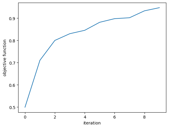
The objective function increased steadily.
[23]:
plt.plot(objective_history)
plt.xlabel("iteration")
plt.ylabel("objective function")
plt.show()
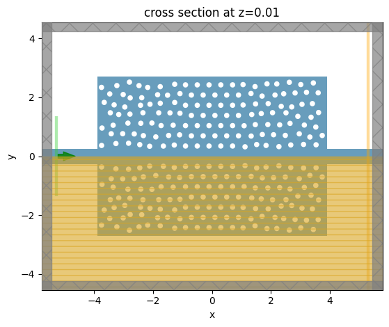
We can grab the last simulation from the parameter history and visualize the fields and flux values over the full spectrum.
[24]:
params_final = param_history[-1]

sim_final = make_sim(params_final, optimization_mode=False)
_ = sim_final.plot(z=0.01)
plt.show()
[25]:
sim_data_final = web.run(sim_final, task_name="phc")
12:27:49 CET Created task 'phc' with resource_id
             'fdve-273e0846-8ad3-476f-b9b8-f0345f5b2cae' and task_type 'FDTD'.
             View task using web UI at
             'https://tidy3d.simulation.cloud/workbench?taskId=fdve-273e0846-8ad
             3-476f-b9b8-f0345f5b2cae'.
Task folder: 'default'.
12:27:59 CET Estimated FlexCredit cost: 0.252. Minimum cost depends on task
             execution details. Use 'web.real_cost(task_id)' to get the billed
             FlexCredit cost after a simulation run.
12:28:01 CET status = queued
             To cancel the simulation, use 'web.abort(task_id)' or
             'web.delete(task_id)' or abort/delete the task in the web UI.
             Terminating the Python script will not stop the job running on the
             cloud.
12:28:10 CET status = preprocess
12:28:16 CET starting up solver
running solver
12:28:48 CET early shutoff detected at 16%, exiting.
12:28:49 CET status = success
             View simulation result at
             'https://tidy3d.simulation.cloud/workbench?taskId=fdve-273e0846-8ad
             3-476f-b9b8-f0345f5b2cae'.
12:28:53 CET Loading results from simulation_data.hdf5
[26]:
_, (ax1, ax2) = plt.subplots(1, 2, tight_layout=True, figsize=(10, 4))
# vmax = 30

ax1 = sim_data0.plot_field("field", field_name="Ey", val="abs", ax=ax1)
ax2 = sim_data_final.plot_field("field", field_name="Ey", val="abs", ax=ax2)
ax1.set_title("original")
ax2.set_title("optimized")
plt.show()
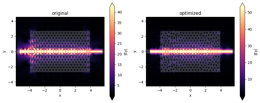
The optimized fields look much smoother, with far less reflection from the input ports.
[27]:
flux_final = abs(sim_data_final["flux"].flux)

flux0.plot(x="f", label="original")
flux_final.plot(x="f", label="optimized")

plt.ylim([0, 1])
plt.title("transmission")
plt.plot([freq0, freq0], [0, 1], linestyle="--", label="optimization freq")

plt.legend()
plt.show()
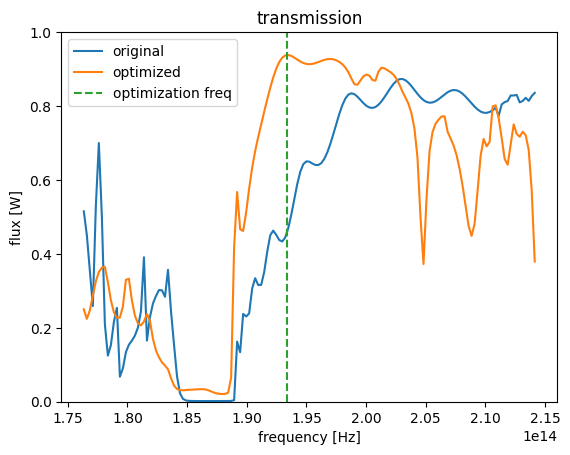
And the new transmission (orange) is far higher above the bandgap, meaning that this new device is coupling light much better from the input waveguide!