Inverse design optimization of a waveguide taper#
In this notebook, we will show how to use tidy3d to optimize a taper with respect to the boundaries of a structure defined using a PolySlab.
We will apply this capability to design a non-adiabatic waveguide taper between a narrow and wide waveguide, based loosely on Michaels, Andrew, and Eli Yablonovitch. "Leveraging continuous material averaging for inverse electromagnetic design." Optics express 26.24 (2018): 31717-31737.
We start by importing our typical python packages, plus tidy3d and autograd.
[41]:
import autograd as ag
import autograd.numpy as anp
import matplotlib.pylab as plt
import numpy as np
import tidy3d as td
import tidy3d.web as web
Set up#
Next we will define some basic parameters of the waveguide, such as the input and output waveguide dimensions, taper width, and taper length.
[42]:
wavelength = 1.0
freq0 = td.C_0 / wavelength

wg_width_in = 0.5 * wavelength
wg_width_out = 5.0 * wavelength

wg_medium = td.material_library["Si3N4"]["Philipp1973Sellmeier"]

wg_length = 1 * wavelength
taper_length = 10.0

spc_pml = 1.5 * wavelength

Lx = wg_length + taper_length + wg_length
Ly = spc_pml + max(wg_width_in, wg_width_out) + spc_pml
Our taper is defined as a set of num_points connected vertices in a polygon. We define the fixed x positions of each vertex and then construct the y positions for the starting device (linear taper).
[43]:
num_points = 101
x_start = -taper_length / 2
x_end = +taper_length / 2
xs = np.linspace(x_start, x_end, num_points)

ys0 = (wg_width_in + (wg_width_out - wg_width_in) * (xs - x_start) / (x_end - x_start)) / 2.0
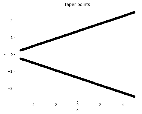
Let’s plot these points to make sure they seem reasonable.
[44]:
plt.plot(xs, +ys0, "ko-")
plt.plot(xs, -ys0, "ko-")
plt.xlabel("x")
plt.ylabel("y")
plt.title("taper points")
plt.show()
Let’s wrap this in a function that constructs these points and then creates a td.PolySlab for use in the td.Simulation.
[45]:
def make_taper(ys) -> td.PolySlab:
    """Create a PolySlab for the taper based on the supplied y values."""
    vertices = anp.concatenate(
        [
            anp.column_stack((xs, ys)),
            anp.column_stack((xs[::-1], -ys[::-1])),
        ]
    )
    return td.PolySlab(vertices=vertices, slab_bounds=(-td.inf, +td.inf), axis=2)
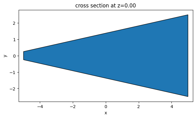
Now we’ll call this function and plot the geometry for a sanity check.
[46]:
# sanity check to see the polyslab
taper_geo = make_taper(ys0)
ax = taper_geo.plot(z=0)
Next, let’s write a function that generates a td.Simulation given a set of y coordinates for the taper, including the monitors, sources, and waveguide geometries.
[47]:
def make_sim(ys, include_field_mnt: bool = False) -> td.Simulation:
    """Make a td.Simulation containing the taper."""

    wg_in_box = td.Box.from_bounds(
        rmin=(-Lx, -wg_width_in / 2, -td.inf),
        rmax=(-Lx / 2 + wg_length + 0.01, +wg_width_in / 2, +td.inf),
    )

    wg_out_box = td.Box.from_bounds(
        rmin=(+Lx / 2 - wg_length - 0.01, -wg_width_out / 2, -td.inf),
        rmax=(+Lx, +wg_width_out / 2, +td.inf),
    )

    taper_geo = make_taper(ys)

    wg_in = td.Structure(geometry=wg_in_box, medium=wg_medium)
    wg_out = td.Structure(geometry=wg_out_box, medium=wg_medium)
    taper = td.Structure(geometry=taper_geo, medium=wg_medium)

    mode_source = td.ModeSource(
        center=(-Lx / 2 + wg_length / 2, 0, 0),
        size=(0, td.inf, td.inf),
        source_time=td.GaussianPulse(freq0=freq0, fwidth=freq0 / 10),
        direction="+",
    )

    mode_monitor = td.ModeMonitor(
        center=(+Lx / 2 - wg_length / 2, 0, 0),
        size=(0, td.inf, td.inf),
        freqs=[freq0],
        mode_spec=td.ModeSpec(),
        name="mode",
    )

    field_monitor = td.FieldMonitor(
        center=(0, 0, 0),
        size=(td.inf, td.inf, 0),
        freqs=[freq0],
        name="field",
    )

    return td.Simulation(
        size=(Lx, Ly, 0),
        structures=[taper, wg_in, wg_out],
        monitors=[mode_monitor, field_monitor] if include_field_mnt else [mode_monitor],
        sources=[mode_source],
        run_time=100 / freq0,
        grid_spec=td.GridSpec.auto(min_steps_per_wvl=20),
        boundary_spec=td.BoundarySpec.pml(x=True, y=True, z=False),
        symmetry=(0, +1, 0),
    )
[48]:
sim = make_sim(ys0)
ax = sim.plot(z=0)
Defining Objective#
Now that we have a function to create our td.Simulation, we need to define our objective function.
We will try to optimize the power transmission into the fundamental mode on the output waveguide, so we write a function to postprocess a td.SimulationData to give this result.
[49]:
def measure_transmission(sim_data: td.SimulationData) -> float:
    """Measure the first order transmission."""
    amp_data = sim_data["mode"].amps
    amp = amp_data.sel(f=freq0, direction="+", mode_index=0).values
    return anp.sum(abs(amp) ** 2)
Next, we will define a few convenience functions to generate our taper y values passed on our objective function parameters.
We define a set of parameters that can range from -infinity to +infinity, but project onto the range [wg_width_out and wg_width_in] through a tanh() function.
We do this to constrain the taper values within this range in a smooth and differentiable way.
We also write an inverse function to get the parameters given a set of desired y values and assert that this function works properly.
[50]:
def get_ys(parameters: np.ndarray) -> np.ndarray:
    """Convert arbitrary parameters to y values for the vertices (parameter (-inf, inf) -> wg width of (wg_width_out, wg_width_in)."""

    params_between_0_1 = (anp.tanh(np.pi * parameters) + 1.0) / 2.0

    params_scaled = params_between_0_1 * (wg_width_out - wg_width_in) / 2.0
    ys = params_scaled + wg_width_in / 2
    return ys


def get_params(ys: np.ndarray) -> np.ndarray:
    """inverse of above, get parameters from ys"""
    params_scaled = ys - wg_width_in / 2
    params_between_0_1 = 2 * params_scaled / (wg_width_out - wg_width_in)
    tanh_pi_params = 2 * params_between_0_1 - 1
    params = np.arctanh(tanh_pi_params) / np.pi
    return params


# assert that the inverse function works properly
np.random.seed(0)  # fix a random seed for reproducibility
params_test = 2 * (np.random.random((10,)) - 0.5)
ys_test = get_ys(params_test)
assert np.allclose(get_params(ys_test), params_test)
We then make a function that simply wraps our previously defined functions to generate a Simulation given some parameters.
[51]:
def make_sim_params(parameters: np.ndarray, include_field_mnt: bool = False) -> td.Simulation:
    """Make the simulation out of raw parameters."""
    ys = get_ys(parameters)
    return make_sim(ys, include_field_mnt=include_field_mnt)
Smoothness Penalty#
It is important to ensure that the final device does not contain feature sizes below a minimum radius of curvature, otherwise there could be considerable difficulty in fabricating the device reliably.
For this, the autograd plugin introduces a penalty function that approximates the radius of curvature about each vertex and introduces a significant penalty to the objective function if that value is below a minimum radius of curvature.
The local radii are determined by fitting a quadratic Bezier curve to each set of 3 adjacent points in the taper and analytically computing the radius of curvature from that curve fit. The details of this calculation are described in the paper linked at the introduction of this notebook.
[52]:
from tidy3d.plugins.autograd import make_curvature_penalty

curvature_penalty = make_curvature_penalty(min_radius=0.15)


def penalty(params: np.ndarray) -> float:
    """Compute penalty for a set of parameters."""
    ys = get_ys(params)
    points = anp.array([xs, ys]).T
    return curvature_penalty(points)
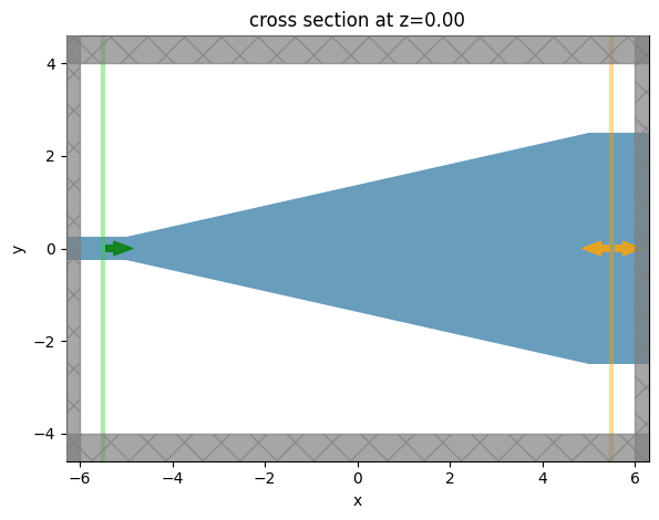
Initial Starting Design#
As our initial design, we take a linear taper between the two waveguides.
[53]:
# desired ys
ys0 = np.linspace(wg_width_in / 2 + 0.001, wg_width_out / 2 - 0.001, num_points)
# corresponding parameters
params0 = get_params(ys0)
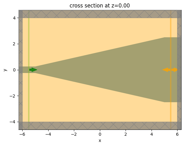
# make the simulation corresponding to these parameters
sim = make_sim_params(params0, include_field_mnt=True)
ax = sim.plot(z=0)
Lets get the penalty value corresponding to this design, which is 0 because the edges are straight (infinite radius of curvature).
[54]:
penalty_value = penalty(params0)
print(f"starting penalty = {float(penalty_value):.2e}")
starting penalty = 0.00e+00
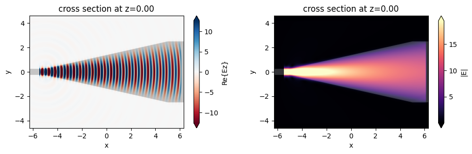
Finally, let’s run this simulation to get a feeling for the initial device performance.
[55]:
sim_data = web.run(sim, task_name="taper fields")
12:22:25 CET Created task 'taper fields' with resource_id
             'fdve-6022f2ab-2d96-4279-9ac8-719698787884' and task_type 'FDTD'.
             View task using web UI at
             'https://tidy3d.simulation.cloud/workbench?taskId=fdve-6022f2ab-2d9
             6-4279-9ac8-719698787884'.
Task folder: 'default'.
12:22:35 CET Estimated FlexCredit cost: 0.025. Minimum cost depends on task
             execution details. Use 'web.real_cost(task_id)' to get the billed
             FlexCredit cost after a simulation run.
12:22:37 CET status = success
12:22:41 CET Loading results from simulation_data.hdf5
[56]:
f, (ax1, ax2) = plt.subplots(1, 2, tight_layout=True, figsize=(10, 3))
sim_data.plot_field(field_monitor_name="field", field_name="Ez", val="real", ax=ax1)
sim_data.plot_field(field_monitor_name="field", field_name="E", val="abs", ax=ax2)
plt.show()
Gradient-based Optimization#
Now that we have our design and post processing functions set up, we are finally ready to put everything together to start optimizing our device with inverse design.
We first set up an objective function that takes the parameters, sets up and runs the simulation, and returns the transmission minus the penalty of the parameters.
[57]:
def objective(parameters: np.ndarray, verbose: bool = False) -> float:
    """Construct simulation, run, and measure transmission."""
    sim = make_sim_params(parameters, include_field_mnt=False)
    sim_data = web.run(sim, task_name="autograd taper", verbose=verbose)
    return measure_transmission(sim_data) - penalty(parameters)
To test our our objective, we will use autograd to make and run a function that returns the objective value and its gradient.
[58]:
grad_fn = ag.value_and_grad(objective)
[59]:
val, grad = grad_fn(params0, verbose=True)
12:22:42 CET Created task 'autograd taper' with resource_id
             'fdve-b3425ea4-1bfa-4f48-aadc-f80b189e73f7' and task_type 'FDTD'.
             View task using web UI at
             'https://tidy3d.simulation.cloud/workbench?taskId=fdve-b3425ea4-1bf
             a-4f48-aadc-f80b189e73f7'.
Task folder: 'default'.
12:23:04 CET Estimated FlexCredit cost: 0.025. Minimum cost depends on task
             execution details. Use 'web.real_cost(task_id)' to get the billed
             FlexCredit cost after a simulation run.
12:23:06 CET status = success
12:23:08 CET Loading results from simulation_data.hdf5
12:23:09 CET Started working on Batch containing 1 tasks.
12:23:28 CET Maximum FlexCredit cost: 0.025 for the whole batch.
             Use 'Batch.real_cost()' to get the billed FlexCredit cost after
             completion.
12:23:30 CET Batch complete.
[60]:
print(f"objective = {val:.2e}")
print(f"gradient = {np.nan_to_num(grad)}")
objective = 7.22e-01
gradient = [ 2.70402303e-03  1.07128122e-01  5.41820996e-02 -1.32454497e-01
 -2.59992656e-01 -3.48714313e-01 -4.03998182e-01 -3.22293757e-01
 -2.18156430e-01 -9.74328450e-02  1.15329957e-01  1.63678384e-01
  3.99418250e-02  9.44981031e-03  8.64775137e-02  2.30880107e-01
  3.37801995e-01  3.80945264e-01  4.39862013e-01  3.89763760e-01
  2.98213687e-01  2.37541050e-01  1.17873319e-01  9.35317544e-02
  1.13871629e-01  4.74236733e-02  1.15292484e-02 -2.55772871e-02
 -5.54620610e-02 -4.34194248e-02 -3.63973435e-02  6.54612285e-03
  3.38436872e-02  3.45213569e-02  4.48255996e-02  3.05782097e-02
  3.94225481e-02  5.09957020e-02  2.53907373e-02  1.13215011e-02
 -4.94807095e-03 -3.14241865e-02 -4.09715824e-02 -3.95352046e-02
 -4.24193762e-02 -4.34819144e-02 -4.03933496e-02 -3.74456215e-02
 -2.66491150e-02 -2.35548218e-02 -2.51762926e-02 -2.72028704e-02
 -3.77861239e-02 -3.86510038e-02 -4.49149180e-02 -4.96946042e-02
 -4.57724967e-02 -5.25367660e-02 -4.47021206e-02 -4.03439921e-02
 -4.41506393e-02 -3.80732654e-02 -4.39680413e-02 -4.31429216e-02
 -4.16956422e-02 -4.67373419e-02 -4.02475470e-02 -4.11541066e-02
 -3.87753984e-02 -3.37245883e-02 -3.64773928e-02 -3.34601885e-02
 -3.29824291e-02 -3.17404463e-02 -2.87530914e-02 -2.78342156e-02
 -2.44293660e-02 -2.39440314e-02 -2.25017021e-02 -2.05562685e-02
 -1.93001185e-02 -1.67661321e-02 -1.55199361e-02 -1.36356589e-02
 -1.28375599e-02 -1.12738294e-02 -9.58097045e-03 -8.99123581e-03
 -6.91170224e-03 -6.56228570e-03 -5.46015962e-03 -4.11763863e-03
 -3.73792906e-03 -2.40056189e-03 -2.21973599e-03 -1.45611445e-03
 -7.77918453e-04 -7.02935222e-04 -1.63798408e-04 -1.00650223e-04
 -2.56740297e-06]
Now we can run Tidy3D’s Adam optimization helpers with this value_and_grad() function. See tutorial 3 for more details on the implementation.
[61]:
from tidy3d.plugins.autograd import adam, optimize

# turn off warnings to reduce verbosity
# td.config.logging.level = "ERROR"

# hyperparameters
num_steps = 50
learning_rate = 0.0075

# initialize adam optimizer with starting parameters
params = np.array(params0).copy()
optimizer = adam(learning_rate=learning_rate)

# store history
objective_history = []
param_history = [np.array(params)]


def record_step(current_params, grad, state, step_index, objective_val):
    print(f"step = {step_index + 1}")
    print(f"\tJ = {objective_val:.4e}")
    print(f"\tgrad_norm = {np.linalg.norm(grad):.4e}")

    objective_history.append(objective_val)
    param_history.append(current_params.copy())


# optimize() minimizes, so maximize J by minimizing -J.
params, opt_state, history = optimize(
    objective,
    params0=params,
    optimizer=optimizer,
    num_steps=num_steps,
    callback=record_step,
    direction="max",
)
param_history.append(params)
step = 1
        J = 7.2187e-01
        grad_norm = 1.2287e+00
step = 2
        J = 7.5440e-01
        grad_norm = 2.6819e+00
step = 3
        J = 7.9931e-01
        grad_norm = 3.8704e+00
step = 4
        J = 8.3137e-01
        grad_norm = 3.1617e+00
step = 5
        J = 8.6354e-01
        grad_norm = 3.3209e+00
step = 6
        J = 8.9107e-01
        grad_norm = 2.0924e+00
step = 7
        J = 8.9329e-01
        grad_norm = 4.1083e+00
step = 8
        J = 9.0966e-01
        grad_norm = 2.8087e+00
step = 9
        J = 9.1510e-01
        grad_norm = 4.3849e+00
step = 10
        J = 9.3508e-01
        grad_norm = 3.0730e+00
step = 11
        J = 9.3369e-01
        grad_norm = 3.6567e+00
step = 12
        J = 9.4278e-01
        grad_norm = 4.1626e+00
step = 13
        J = 9.5260e-01
        grad_norm = 3.2437e+00
step = 14
        J = 9.5019e-01
        grad_norm = 4.1740e+00
step = 15
        J = 9.5787e-01
        grad_norm = 3.4446e+00
step = 16
        J = 9.6512e-01
        grad_norm = 2.8349e+00
step = 17
        J = 9.6442e-01
        grad_norm = 3.9073e+00
step = 18
        J = 9.7087e-01
        grad_norm = 2.6403e+00
step = 19
        J = 9.7459e-01
        grad_norm = 2.2828e+00
step = 20
        J = 9.7596e-01
        grad_norm = 2.1056e+00
step = 21
        J = 9.7539e-01
        grad_norm = 2.5387e+00
step = 22
        J = 9.7776e-01
        grad_norm = 2.3652e+00
step = 23
        J = 9.8137e-01
        grad_norm = 1.6393e+00
step = 24
        J = 9.8308e-01
        grad_norm = 1.2322e+00
step = 25
        J = 9.8286e-01
        grad_norm = 2.1248e+00
step = 26
        J = 9.8406e-01
        grad_norm = 1.5221e+00
step = 27
        J = 9.8542e-01
        grad_norm = 1.5841e+00
step = 28
        J = 9.8754e-01
        grad_norm = 1.3093e+00
step = 29
        J = 9.8801e-01
        grad_norm = 1.4603e+00
step = 30
        J = 9.8890e-01
        grad_norm = 1.4407e+00
step = 31
        J = 9.9032e-01
        grad_norm = 9.4141e-01
step = 32
        J = 9.9041e-01
        grad_norm = 1.2397e+00
step = 33
        J = 9.9144e-01
        grad_norm = 9.6688e-01
step = 34
        J = 9.9254e-01
        grad_norm = 8.1483e-01
step = 35
        J = 9.9260e-01
        grad_norm = 1.0262e+00
step = 36
        J = 9.9319e-01
        grad_norm = 9.0639e-01
step = 37
        J = 9.9381e-01
        grad_norm = 9.0826e-01
step = 38
        J = 9.9432e-01
        grad_norm = 5.4159e-01
step = 39
        J = 9.9430e-01
        grad_norm = 8.4398e-01
step = 40
        J = 9.9500e-01
        grad_norm = 4.2442e-01
step = 41
        J = 9.9470e-01
        grad_norm = 8.0397e-01
step = 42
        J = 9.9511e-01
        grad_norm = 5.4018e-01
step = 43
        J = 9.9539e-01
        grad_norm = 5.3265e-01
step = 44
        J = 9.9562e-01
        grad_norm = 4.4275e-01
step = 45
        J = 9.9600e-01
        grad_norm = 3.0932e-01
step = 46
        J = 9.9611e-01
        grad_norm = 3.8814e-01
step = 47
        J = 9.9633e-01
        grad_norm = 3.6916e-01
step = 48
        J = 9.9676e-01
        grad_norm = 2.5210e-01
step = 49
        J = 9.9694e-01
        grad_norm = 2.6960e-01
step = 50
        J = 9.9712e-01
        grad_norm = 2.1953e-01
[62]:
params_best = param_history[-1]
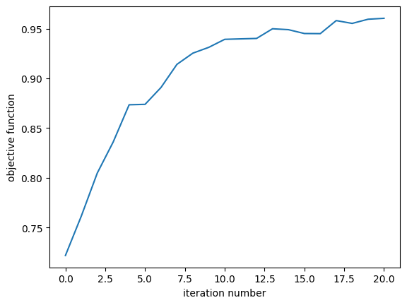
We see that our objective has increased steadily from a transmission of 56% to about 95%!
[63]:
ax = plt.plot(objective_history)
plt.xlabel("iteration number")
plt.ylabel("objective function")
plt.show()
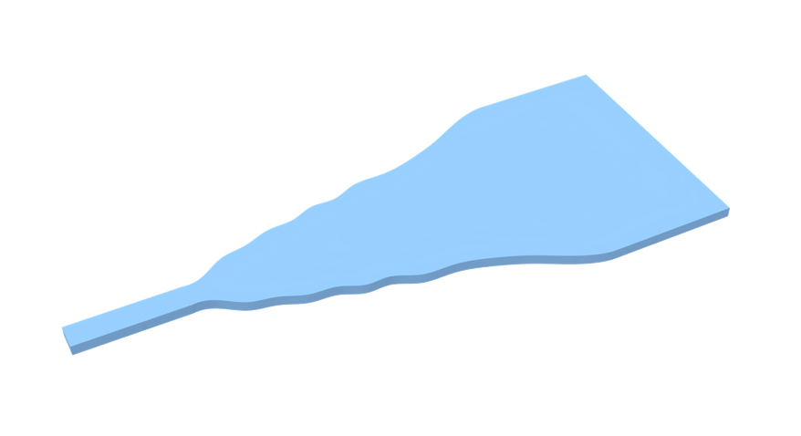
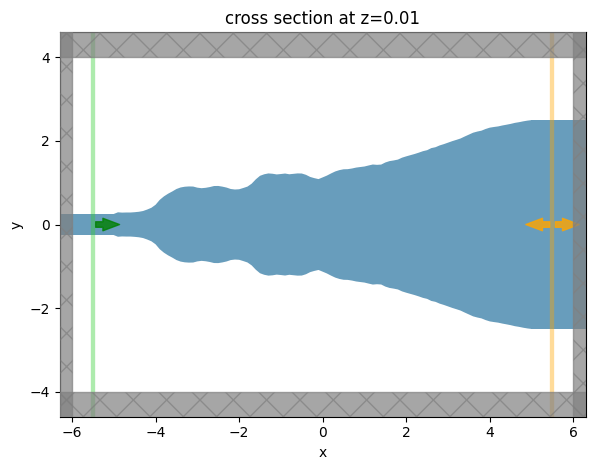
Our final device displays smooth features and no sharp corners. Without our penalty this would have not been the case!
[64]:
sim_best = make_sim_params(param_history[-1], include_field_mnt=True)
ax = sim_best.plot(z=0.01)
[65]:
sim_data_best = td.web.run(sim_best, task_name="taper final")
13:37:25 CET Created task 'taper final' with resource_id
             'fdve-a88910ab-50bb-46f1-9a37-f0658dc89367' and task_type 'FDTD'.
             View task using web UI at
             'https://tidy3d.simulation.cloud/workbench?taskId=fdve-a88910ab-50b
             b-46f1-9a37-f0658dc89367'.
Task folder: 'default'.
13:37:52 CET Estimated FlexCredit cost: 0.025. Minimum cost depends on task
             execution details. Use 'web.real_cost(task_id)' to get the billed
             FlexCredit cost after a simulation run.
13:37:54 CET status = queued
             To cancel the simulation, use 'web.abort(task_id)' or
             'web.delete(task_id)' or abort/delete the task in the web UI.
             Terminating the Python script will not stop the job running on the
             cloud.
13:38:20 CET starting up solver
13:38:21 CET running solver
13:38:22 CET early shutoff detected at 48%, exiting.
13:38:23 CET status = success
             View simulation result at
             'https://tidy3d.simulation.cloud/workbench?taskId=fdve-a88910ab-50b
             b-46f1-9a37-f0658dc89367'.
13:38:30 CET Loading results from simulation_data.hdf5
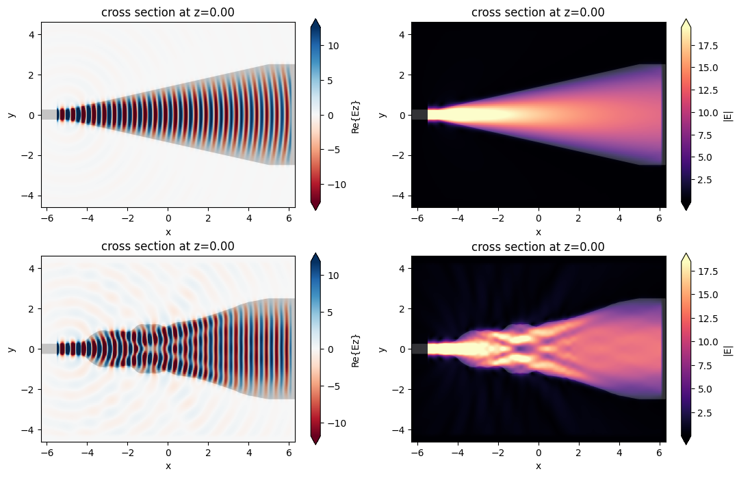
Comparing the field patterns, we see that the optimized device gives a much more uniform field profile at the output waveguide, as desired. One can further check that this device and field pattern matches the referenced paper quite nicely!
[66]:
f, ((ax1, ax2), (ax3, ax4)) = plt.subplots(2, 2, tight_layout=True, figsize=(11, 7))

# plot original
sim_data.plot_field(field_monitor_name="field", field_name="Ez", val="real", ax=ax1)
sim_data.plot_field(field_monitor_name="field", field_name="E", val="abs", ax=ax2)

# plot optimized
sim_data_best.plot_field(field_monitor_name="field", field_name="Ez", val="real", ax=ax3)
sim_data_best.plot_field(field_monitor_name="field", field_name="E", val="abs", ax=ax4)

plt.show()
[67]:
transmission_start = float(measure_transmission(sim_data))
transmission_end = float(measure_transmission(sim_data_best))
print(
    f"Transmission improved from {(transmission_start * 100):.2f}% to {(transmission_end * 100):.2f}%"
)
Transmission improved from 72.19% to 99.77%