

Bayesian optimization of a Y branch#
Note: the cost of running the entire notebook is larger than 10 FlexCredits.
Bayesian optimization is a popular technique for searching and optimizing a design space. It works by building a probabilistic model, such as a Gaussian process, to predict the outcome of a more complex objective function. Unlike other optimizers like genetic algorithms or particle swarm optimization, Bayesian optimization uses an acquisition function to select new potential solutions, focusing on areas of the design space that the Gaussian process predicts will have high objective values and high uncertainty. Over the course of the optimization, the model’s uncertainty reduces, improving its accuracy as a surrogate for the true objective function. This makes Bayesian optimization a direct approach to optimization, particularly well-suited to problems with small (< 30 dimensions) and expensive-to-evaluate objective functions.
However, as Bayesian optimization is an iterative process with many individual components, it can be challenging to design and parallelize, leading to long run times and high computational costs. Fortunately, the Design plugin in Tidy3D includes the Bayesian optimization method MethodBayOpt which eliminates much of this complexity. Users can quickly and easily run a Bayesian optimization for complex FDTD simulations and analyze the results. Further details on Bayesian optimization and
the methods used in Tidy3D are available in the open-source Python library bayesian_optimization.
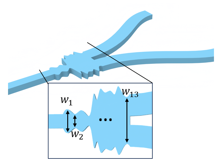
This notebook details how to perform a Bayesian optimization with the Tidy3D Design plugin for the development of a Y-junction. It is based on the work of Zhengqi Gao, Zhengxing Zhang, and Duane S. Boning, "Automatic Synthesis of Broadband Silicon Photonic Devices via Bayesian Optimization" Journal of Lightwave Technology 40, 7879-7892 (2022) DOI:10.1109/JLT.2022.3207052. A detailed description of how to build a Y-junction can be found in
the Waveguide Y junction.
If you are curious about other Design plugin features, see these notebooks:
[1]:
# The Bayesian optimizer uses the bayesian-optimization external package version 1.5.1.
# Uncomment the following line to install the package
# pip install bayesian-optimization==1.5.1

import gdstk
import matplotlib.pyplot as plt
import numpy as np
import tidy3d as td
import tidy3d.plugins.design as tdd
import tidy3d.web as web
from scipy.interpolate import make_interp_spline
Simulation Setup#
The simulation is defined across the 1.5 \(\mu m\) to 1.6 \(\mu m\) wavelength range with 100 sampling points. The base of the model is silicon, the top of the model is silicon dioxide; we use the material constants included in the Tidy3D Tidy3D’s material library.
[2]:
lda0 = 1.55  # central wavelength
freq0 = td.C_0 / lda0  # central frequency
n_wav = 100  # Number of wavelengths to sample in the range
ldas = np.linspace(1.5, 1.6, n_wav)  # wavelength range
freqs = td.C_0 / ldas  # frequency range
fwidth = 0.5 * (np.max(freqs) - np.min(freqs))  # width of the source frequency range

si = td.material_library["cSi"]["Palik_LowLoss"]
sio2 = td.material_library["SiO2"]["Palik_LowLoss"]
The following parameters describe the geometry of the waveguide. The optimizable design space is the junction which is split into 13 discrete segments.
[3]:
t = 0.22  # thickness of the silicon layer
num_d = 13  # dimensional space of the design region

l_in = 1  # input waveguide length
l_junction = 2  # length of the junction
l_bend = 6  # horizontal length of the waveguide bend
h_bend = 2  # vertical offset of the waveguide bend
l_out = 1  # output waveguide length
branch_width = 0.5  # width of one Y branch
branch_sep = 0.2  # distance between y branches at the junction
inf_eff = 100  # effective infinity
The most effective way to use the Design plugin is to split the workflow into “pre” and “post” functions which can surround a call to the Tidy3D cloud that carries out the computation. This takes advantage of automated simulation batching, allowing for parallelization which saves a considerable amount of time. The pre-function returns a Simulation; the post-function then analyzes the corresponding SimulationData. Together they can be considered the fitness function (or objective function
/ figure of merit) which the Bayesian optimization process is working to predict.
The function fn_pre needs to take the parameters that are being optimized: these are the 13 width segments of the junction. They always input as a dictionary and can be unpacked within the function (as below) or included as keyword arguments. These parameters are used to build a Y-junction Simulation object.
The function fn_post then takes the SimulationData object output by the simulation and computes the objective function. The value of objective is then fed back into the Bayesian optimization to inform the probabilistic model. In this case, we extract the power passing through the Y-junction and the power reflected back to the source. These values are evaluated in a custom loss function described by Gao et al. to determine the effectiveness of the junction design:
where the summation is performed over the simulated wavelengths, \(N_\lambda\) is the number of wavelength points, \(R\) is the reflected power and \(T\) is the transmitted power in one branch.
The aim of this function is to achieve a transmitted power of 0.5 through each branch, whilst driving the power reflected towards the source to zero. Note there is a minus sign in front of the output value as this loss function is a minimizing function, whilst all the optimizers in the Design plugin are built to maximize the objective function.
[4]:
def fn_pre(**w_params: dict) -> td.Simulation:
    """Create a Simulation of a Y splitter from a series of junction widths.

    Includes mode monitors to measure the power transmitted and reflected to source.
    """
    w_start = 0.5
    w_end = branch_width * 2 + branch_sep

    widths = [w_start]  # Ensures input waveguide is included in spline for first point of junction
    widths.extend(list(w_params.values()))
    widths.append(w_end)  # Ensures final point of junction smoothly converts to the branches

    x_junction = np.linspace(
        l_in, l_in + l_junction, num_d + 2
    )  # x coordinates of the top edge vertices
    y_junction = np.array(widths)  # y coordinates of the top edge vertices

    # pass vertices through spline and increase sampling to smooth the geometry
    new_x_junction = np.linspace(
        l_in, l_in + l_junction, 100
    )  # x coordinates of the top edge vertices
    spline = make_interp_spline(x_junction, y_junction, k=2)
    spline_yjunction = spline(new_x_junction)

    # using concatenate to include bottom edge vertices
    x_junction = np.concatenate((new_x_junction, np.flipud(new_x_junction)))
    y_junction = np.concatenate((spline_yjunction / 2, -np.flipud(spline_yjunction / 2)))

    # stacking x and y coordinates to form vertices pairs
    vertices = np.transpose(np.vstack((x_junction, y_junction)))

    junction = td.Structure(
        geometry=td.PolySlab(vertices=vertices, axis=2, slab_bounds=(0, t)), medium=si
    )

    x_start = l_in + l_junction  # x coordinate of the starting point of the waveguide bends

    x_bend = np.linspace(x_start, x_start + l_bend, 100)  # x coordinates of the top edge vertices

    y_bend = (
        (x_bend - x_start) * h_bend / l_bend
        - h_bend * np.sin(2 * np.pi * (x_bend - x_start) / l_bend) / (np.pi * 2)
        + w_end / 2
        - w_start / 2
    )  # y coordinates of the top edge vertices

    # adding the last point to include the straight waveguide at the output
    x_bend = np.append(x_bend, inf_eff)
    y_bend = np.append(y_bend, y_bend[-1])

    # add path to the cell
    cell = gdstk.Cell("bends")
    cell.add(
        gdstk.FlexPath(x_bend + 1j * y_bend, branch_width, layer=1, datatype=0)
    )  # top waveguide bend
    cell.add(
        gdstk.FlexPath(x_bend - 1j * y_bend, branch_width, layer=1, datatype=0)
    )  # bottom waveguide bend

    # define top waveguide bend structure
    wg_bend_1 = td.Structure(
        geometry=td.PolySlab.from_gds(
            cell,
            gds_layer=1,
            axis=2,
            slab_bounds=(0, t),
        )[0],
        medium=si,
    )

    # define bottom waveguide bend structure
    wg_bend_2 = td.Structure(
        geometry=td.PolySlab.from_gds(
            cell,
            gds_layer=1,
            axis=2,
            slab_bounds=(0, t),
        )[1],
        medium=si,
    )

    # straight input waveguide
    wg_in = td.Structure(
        geometry=td.Box.from_bounds(rmin=(-inf_eff, -w_start / 2, 0), rmax=(l_in, w_start / 2, t)),
        medium=si,
    )

    # the entire model is the collection of all structures defined so far
    model_structure = [wg_in, junction, wg_bend_1, wg_bend_2]

    Lx = l_in + l_junction + l_out + l_bend  # simulation domain size in x direction
    Ly = w_end + 2 * h_bend + 1.5 * lda0  # simulation domain size in y direction
    Lz = 10 * t  # simulation domain size in z direction
    sim_size = (Lx, Ly, Lz)

    # add a mode source as excitation
    mode_spec = td.ModeSpec(num_modes=1, target_neff=3.5)
    mode_source = td.ModeSource(
        center=(l_in / 2, 0, t / 2),
        size=(0, 4 * w_start, 6 * t),
        source_time=td.GaussianPulse(freq0=freq0, fwidth=fwidth),
        direction="+",
        mode_spec=mode_spec,
        mode_index=0,
    )

    # add a mode monitor to measure transmission at the output waveguide
    mode_monitor_11 = td.ModeMonitor(
        center=(l_in / 3, 0, t / 2),
        size=(0, 4 * w_start, 6 * t),
        freqs=freqs,
        mode_spec=mode_spec,
        name="mode_11",
    )

    mode_monitor_12 = td.ModeMonitor(
        center=(l_in + l_junction + l_bend + l_out / 2, w_end / 2 - w_start / 2 + h_bend, t / 2),
        size=(0, 4 * w_start, 6 * t),
        freqs=freqs,
        mode_spec=mode_spec,
        name="mode_12",
    )

    # add a field monitor to visualize field distribution at z=t/2
    field_monitor = td.FieldMonitor(
        center=(0, 0, t / 2), size=(td.inf, td.inf, 0), freqs=[freq0], name="field"
    )

    run_time = 5e-13  # simulation run time

    # construct simulation
    sim = td.Simulation(
        center=(Lx / 2, 0, 0),
        size=sim_size,
        grid_spec=td.GridSpec.auto(min_steps_per_wvl=20, wavelength=lda0),
        structures=model_structure,
        sources=[mode_source],
        monitors=[mode_monitor_11, mode_monitor_12, field_monitor],
        run_time=run_time,
        boundary_spec=td.BoundarySpec.all_sides(boundary=td.PML()),
        medium=sio2,
    )

    return sim


def fn_post(sim_data: td.SimulationData) -> float:
    """Calculate the loss function from the power at the mode monitors in the SimulationData."""
    # Calculate the power reflected back to source and transmitted to one branch
    power_reflected = np.squeeze(
        np.abs(sim_data["mode_11"].amps.sel(direction="-", mode_index=0)) ** 2
    )
    power_transmitted = np.squeeze(
        np.abs(sim_data["mode_12"].amps.sel(direction="+", mode_index=0)) ** 2
    )

    # Loss function proposed by Gao et al. which takes advantage of branch symmetry
    loss_fn = 1 / 3 * n_wav * np.sum(power_reflected**2 + 2 * (power_transmitted - 0.5) ** 2)
    output = -float(loss_fn.values)  # Negative value as this is a minimizing loss function

    return output
We can quickly check that fn_pre is working correctly by passing a set of potential test_params and plotting the result. Note that the gap between the Polyslab junction and the branches is a plotting artifact and doesn’t exist in the Simulation.
[5]:
test_params = {
    "w1": 0.5,
    "w2": 0.5,
    "w3": 0.6,
    "w4": 0.7,
    "w5": 0.9,
    "w6": 1.26,
    "w7": 1.4,
    "w8": 1.4,
    "w9": 1.4,
    "w10": 1.4,
    "w11": 1.31,
    "w12": 0.5,
    "w13": 0.5,
}
sim = fn_pre(**test_params)
sim.plot(z=0)
plt.show()
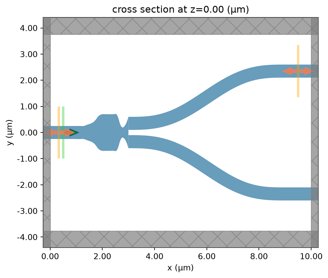
Next, we setup the Bayesian optimization method. This is done with the MethodBayOpt object. We don’t have the lcb (lower confidence bound) acquisition function used in the paper available to us, but by making our loss function negative and using the ucb (upper confidence bound) acquisition we achieve the same optimizer design. The initial_iter and n_iter options control the number of initial random samples and subsequent optimization iterations respectively. We can also set
the random seed to ensure reproducible results (optional).
We also create a list of ParameterFloat objects corresponding to the 13 segment widths. The span option defines the bounds of each parameter.
The method and parameters are then passed to a DesignSpace object which contains all we need to run the Bayesian optimization.
[6]:
method = tdd.MethodBayOpt(
    initial_iter=30,
    n_iter=70,
    acq_func="ucb",
    kappa=0.3,
    seed=1,
)

parameters = [tdd.ParameterFloat(name=f"w_{i}", span=(0.5, 1.6)) for i in range(num_d)]

design_space = tdd.DesignSpace(
    method=method, parameters=parameters, task_name="bay_opt_notebook", path_dir="./data"
)
It is then very easy to the launch this optimization with design_space.run(). This launches an initial random batch of 30 simulations, as specified by initial_iter, followed by sequential computation of 70 simulations, as specified by n_iter. In the latter phase, the Bayesian optimizer chooses potential candidates based on simultaneously maximizing the objective value and efficiently exploring the design space. The total of 100 simulations takes around 90 minutes to compute. Once
complete, the results are returned in a pandas dataframe for analysis.
[7]:
results = design_space.run(fn_pre, fn_post, verbose=True)
df = results.to_dataframe()
07:51:28 UTC Running 30 Simulations
07:53:56 UTC Best Fit from Initial Solutions: -180.654
Running 1 Simulations
07:54:38 UTC Running 1 Simulations
07:55:17 UTC Running 1 Simulations
07:55:57 UTC Latest Best Fit on Iter 2: -150.268
07:55:58 UTC Running 1 Simulations
07:56:39 UTC Latest Best Fit on Iter 3: -134.703
07:56:40 UTC Running 1 Simulations
07:57:20 UTC Latest Best Fit on Iter 4: -122.116
07:57:21 UTC Running 1 Simulations
07:58:23 UTC Running 1 Simulations
07:59:08 UTC Latest Best Fit on Iter 6: -80.47
07:59:09 UTC Running 1 Simulations
08:00:02 UTC Running 1 Simulations
08:00:54 UTC Running 1 Simulations
08:01:31 UTC Running 1 Simulations
08:02:07 UTC Running 1 Simulations
08:02:58 UTC Latest Best Fit on Iter 11: -74.239
08:02:59 UTC Running 1 Simulations
08:03:50 UTC Latest Best Fit on Iter 12: -68.458
08:03:51 UTC Running 1 Simulations
08:04:36 UTC Latest Best Fit on Iter 13: -63.557
Running 1 Simulations
08:05:30 UTC Running 1 Simulations
08:07:40 UTC Running 1 Simulations
08:08:16 UTC Latest Best Fit on Iter 16: -48.535
08:08:18 UTC Running 1 Simulations
08:09:13 UTC Running 1 Simulations
08:09:45 UTC Running 1 Simulations
08:10:41 UTC Running 1 Simulations
08:11:45 UTC Latest Best Fit on Iter 20: -43.538
08:11:46 UTC Running 1 Simulations
08:12:55 UTC Running 1 Simulations
08:13:25 UTC Latest Best Fit on Iter 22: -37.147
08:13:26 UTC Running 1 Simulations
08:14:06 UTC Latest Best Fit on Iter 23: -35.19
Running 1 Simulations
08:15:25 UTC Running 1 Simulations
08:15:59 UTC Running 1 Simulations
08:16:39 UTC Latest Best Fit on Iter 26: -26.814
08:16:40 UTC Running 1 Simulations
08:18:27 UTC Latest Best Fit on Iter 27: -13.14
08:18:28 UTC Running 1 Simulations
08:18:59 UTC Latest Best Fit on Iter 28: -10.107
08:19:00 UTC Running 1 Simulations
08:19:53 UTC Running 1 Simulations
08:20:41 UTC Latest Best Fit on Iter 30: -9.442
08:20:42 UTC Running 1 Simulations
08:22:29 UTC Latest Best Fit on Iter 31: -8.845
08:22:30 UTC Running 1 Simulations
08:23:13 UTC Running 1 Simulations
08:24:03 UTC Running 1 Simulations
08:24:41 UTC Latest Best Fit on Iter 34: -6.618
08:24:42 UTC Running 1 Simulations
08:25:20 UTC Latest Best Fit on Iter 35: -4.252
08:25:21 UTC Running 1 Simulations
08:25:57 UTC Latest Best Fit on Iter 36: -4.168
08:25:58 UTC Running 1 Simulations
08:27:16 UTC Running 1 Simulations
08:27:52 UTC Latest Best Fit on Iter 38: -4.111
08:27:53 UTC Running 1 Simulations
08:29:48 UTC Latest Best Fit on Iter 39: -4.033
08:29:49 UTC Running 1 Simulations
08:31:23 UTC Latest Best Fit on Iter 40: -3.751
08:31:24 UTC Running 1 Simulations
08:32:14 UTC Running 1 Simulations
08:33:04 UTC Latest Best Fit on Iter 42: -3.469
08:33:05 UTC Running 1 Simulations
08:33:39 UTC Latest Best Fit on Iter 43: -3.204
Running 1 Simulations
08:34:18 UTC Latest Best Fit on Iter 44: -2.863
08:34:19 UTC Running 1 Simulations
08:34:52 UTC Latest Best Fit on Iter 45: -2.695
08:34:53 UTC Running 1 Simulations
08:35:46 UTC Running 1 Simulations
08:36:24 UTC Latest Best Fit on Iter 47: -2.631
08:36:25 UTC Running 1 Simulations
08:37:22 UTC Running 1 Simulations
08:38:12 UTC Running 1 Simulations
08:39:02 UTC Latest Best Fit on Iter 50: -2.553
08:39:03 UTC Running 1 Simulations
08:39:57 UTC Running 1 Simulations
08:40:27 UTC Latest Best Fit on Iter 52: -2.352
08:40:28 UTC Running 1 Simulations
08:40:56 UTC Latest Best Fit on Iter 53: -2.299
08:40:57 UTC Running 1 Simulations
08:41:34 UTC Running 1 Simulations
08:42:25 UTC Running 1 Simulations
08:43:13 UTC Running 1 Simulations
08:43:43 UTC Latest Best Fit on Iter 57: -2.294
08:43:44 UTC Running 1 Simulations
08:45:51 UTC Latest Best Fit on Iter 58: -2.201
08:45:52 UTC Running 1 Simulations
08:46:24 UTC Latest Best Fit on Iter 59: -2.161
08:46:25 UTC Running 1 Simulations
08:46:59 UTC Latest Best Fit on Iter 60: -2.151
08:47:00 UTC Running 1 Simulations
08:47:51 UTC Running 1 Simulations
08:48:42 UTC Latest Best Fit on Iter 62: -2.086
08:48:43 UTC Running 1 Simulations
08:49:15 UTC Running 1 Simulations
08:50:07 UTC Running 1 Simulations
08:50:59 UTC Running 1 Simulations
08:51:50 UTC Latest Best Fit on Iter 66: -2.062
08:51:51 UTC Running 1 Simulations
08:52:27 UTC Running 1 Simulations
08:53:18 UTC Running 1 Simulations
08:53:52 UTC Best Result: -2.061516190245546
             Best Parameters: w_0: 0.5498419634833278 w_1: 0.5 w_2:
             1.296267581582306 w_3: 0.8380428776617914 w_4: 1.6 w_5: 1.6 w_6:
             1.6 w_7: 1.452243062356684 w_8: 1.51043959613503 w_9:
             1.4942004790785968 w_10: 1.3010925645718425 w_11: 1.6 w_12:
             1.1789774737217065
Results#
The best result can be extracted directly from the optimizer object. Plotting this, we see what the optimizer has returned as the optimized structure for this design of Y-junction.
[8]:
best_params = results.optimizer.max["params"]
print(f"Best fitness: {results.optimizer.max['target']}")
sim = fn_pre(**best_params)
sim.plot(z=0)
plt.show()
Best fitness: -2.061516190245546
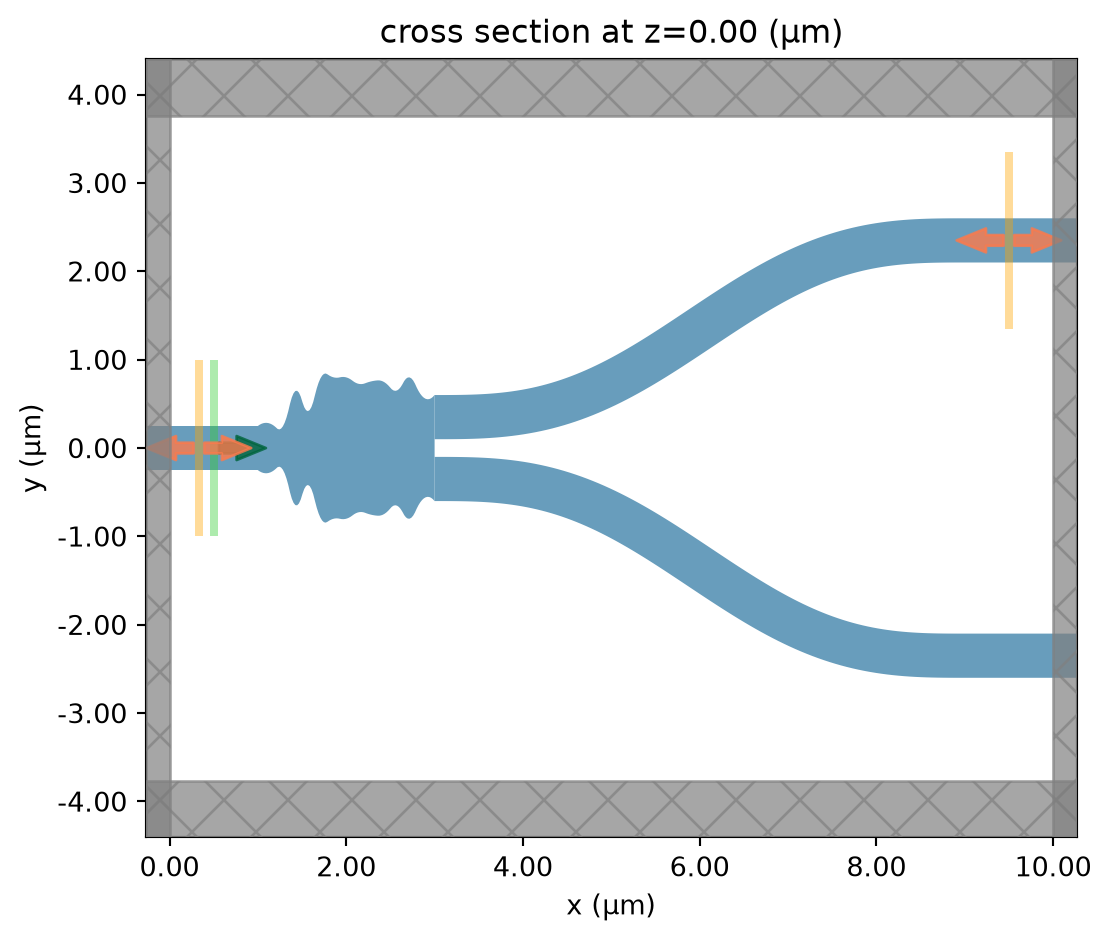
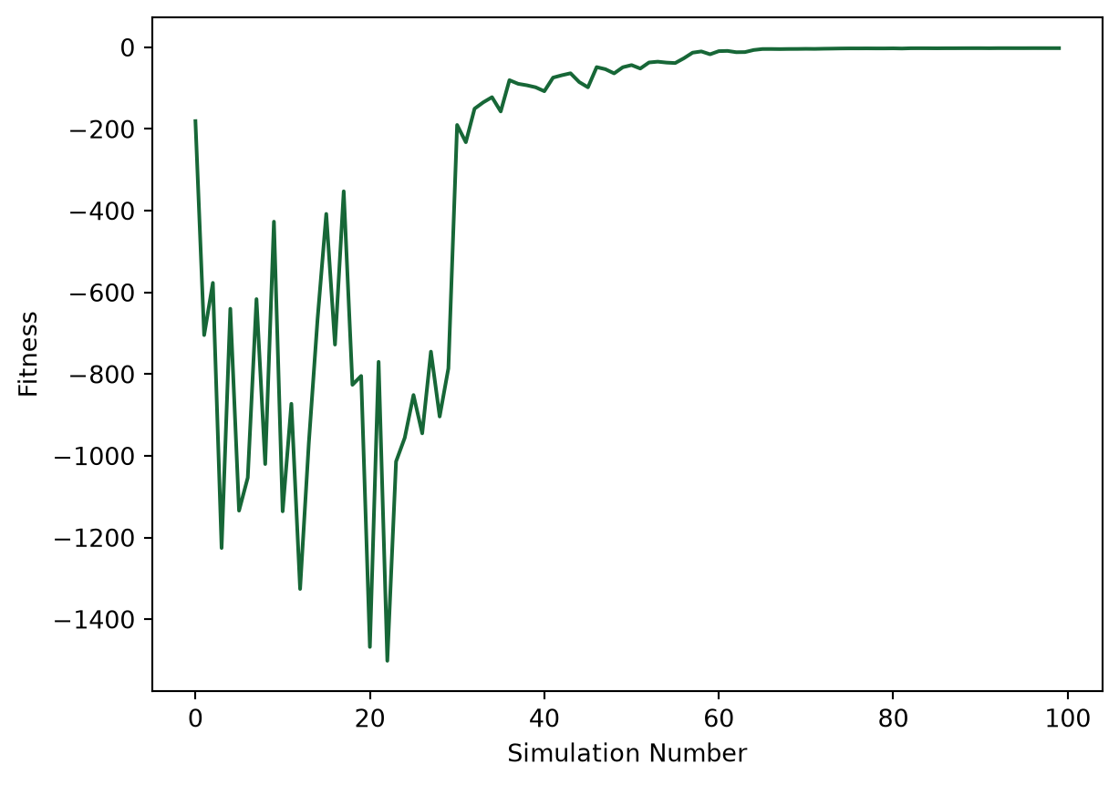
We can then create a plot to evaluate if the Bayesian optimization has converged on a fitness value. The first 30 iterations are from the random initialization, so the fitness values are expected to be more varied. The fitness has converged before the end of the remaining 70 iterations; an early stop criteria could have been included to finish the optimization sooner.
[9]:
ax = df["output"].plot(xlabel="Simulation Number", ylabel="Fitness")
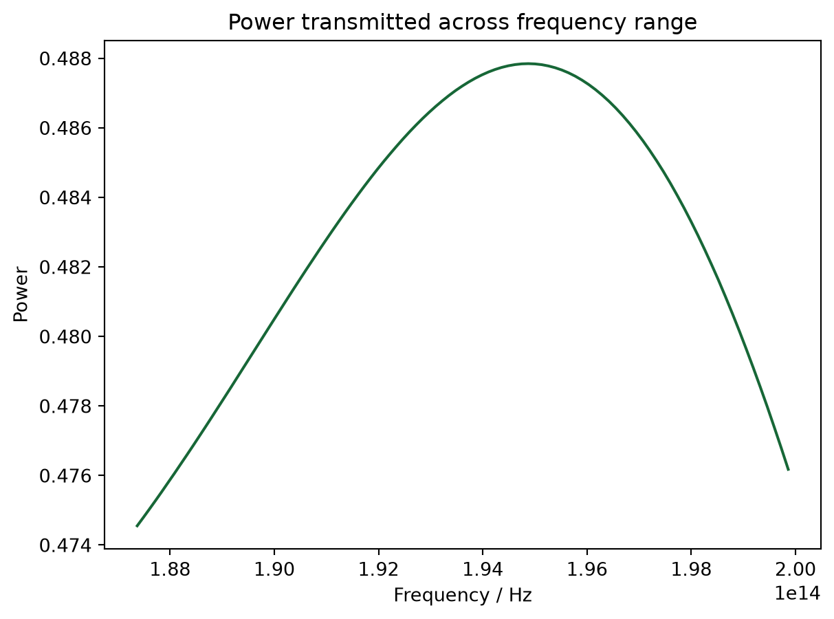
The mean power at the reflected and transmitted monitors can be calculated and compared to the paper from Gao et al.
[10]:
idx_best_result = df["output"].idxmax()
best_sim_filename = results.task_paths[idx_best_result]
best_sim = td.SimulationData.from_file(best_sim_filename)

power_reflected = np.array(
    np.squeeze(np.abs(best_sim["mode_11"].amps.sel(direction="-", mode_index=0)) ** 2)
).mean()
power_transmitted = np.array(
    np.squeeze(np.abs(best_sim["mode_12"].amps.sel(direction="+", mode_index=0)) ** 2)
).mean()

print(f"Mean Reflected Power: {round(power_reflected, 3)} (Paper: 0.004)")
print(f"Mean Transmitted Power: {round(power_transmitted, 3)} (Paper: 0.460)")
Mean Reflected Power: 0.001 (Paper: 0.004)
Mean Transmitted Power: 0.483 (Paper: 0.460)
Final Optimized Design#
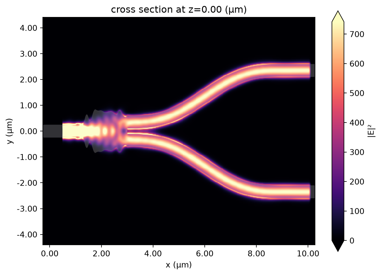
Finally, we can simulate the optimal solution with an additional FieldMonitor to visualise the field distribution throughout the splitter.
[11]:
final_sim = fn_pre(**best_params)

# Define a field monitor to help visualize the field distribution
field_monitor = td.FieldMonitor(
    center=(0, 0, 0), size=(td.inf, td.inf, 0), freqs=[freq0], name="field"
)

mode_12 = final_sim.monitors[1]

final_sim = final_sim.copy(update={"monitors": (field_monitor, mode_12)})

final_sim_data = web.run(final_sim, task_name="BO_notebook_final_sim")
08:53:53 UTC Created task 'BO_notebook_final_sim' with resource_id
             'fdve-954d6d79-e621-480f-90d7-1898454dc380' and task_type 'FDTD'.
             View task using web UI at
             'https://tidy3d.simulation.cloud/workbench?taskId=fdve-954d6d79-e62
             1-480f-90d7-1898454dc380'.
Task folder: 'default'.
08:53:54 UTC Estimated FlexCredit cost: 0.115. This assumes the FDTD solver runs
             for the full simulation time; if early shutoff is reached, the
             billed cost can be lower. Use 'web.real_cost(task_id)' to get the
             billed FlexCredit cost after a simulation run.
08:53:59 UTC status = queued
             To cancel the simulation, use 'web.abort(task_id)' or
             'web.delete(task_id)' or abort/delete the task in the web UI.
             Terminating the Python script will not stop the job running on the
             cloud.
08:54:06 UTC status = preprocess
08:54:11 UTC starting up solver
running solver
08:54:19 UTC early shutoff detected at 76%, exiting.
08:54:20 UTC status = postprocess
08:54:22 UTC status = success
08:54:24 UTC View simulation result at
             'https://tidy3d.simulation.cloud/workbench?taskId=fdve-954d6d79-e62
             1-480f-90d7-1898454dc380'.
08:54:26 UTC Loading results from simulation_data.hdf5
Plotting the field shows how it splits evenly between each branch.
[12]:
final_sim_data.plot_field("field", "E", "abs^2")
plt.show()
And we can visualise how the power transmitted varies over the frequency range.
[13]:
power_transmitted = np.squeeze(
    np.abs(final_sim_data["mode_12"].amps.sel(direction="+", mode_index=0)) ** 2
)
plt.plot(freqs, power_transmitted)
plt.title("Power transmitted across frequency range")
plt.xlabel("Frequency / Hz")
plt.ylabel("Power")
plt.show()
Conclusion#
Through comparison of the junction geometry and the transmitted and reflected power, we can show that these results closely follow the results published by Gao et al. for the design of a Y-junction. This notebook demonstrates how to carry out Bayesian optimization with the Design plugin, and can be readily adapted to other use cases.
Learn more about the Design plugin: