tidy3d.components.simulation.AbstractYeeGridSimulation#
- class AbstractYeeGridSimulation[source]#
Bases:
AbstractSimulation,ABCAbstract class for a simulation involving electromagnetic fields defined on a Yee grid.
- Parameters:
center (tuple[Union[float, autograd.tracer.Box], Union[float, autograd.tracer.Box], Union[float, autograd.tracer.Box]] = (0.0, 0.0, 0.0)) – [units = um]. Center of object in x, y, and z.
size (tuple[Union[NonNegativeFloat, autograd.tracer.Box], Union[NonNegativeFloat, autograd.tracer.Box], Union[NonNegativeFloat, autograd.tracer.Box]]) – [units = um]. Size in x, y, and z directions.
medium (Union[
Medium,AnisotropicMedium,PECMedium,PMCMedium,PoleResidue,Sellmeier,Lorentz,Debye,Drude,FullyAnisotropicMedium,CustomMedium,CustomPoleResidue,CustomSellmeier,CustomLorentz,CustomDebye,CustomDrude,CustomAnisotropicMedium,PerturbationMedium,PerturbationPoleResidue,LossyMetalMedium] = Medium()) – Background medium of simulation, defaults to vacuum if not specified.structures (tuple[
Structure, …] = ()) – Tuple of structures present in simulation. Note: Structures defined later in this list override the simulation material properties in regions of spatial overlap.symmetry (tuple[Literal[0, -1, 1], Literal[0, -1, 1], Literal[0, -1, 1]] = (0, 0, 0)) – Tuple of integers defining reflection symmetry across a plane bisecting the simulation domain normal to the x-, y-, and z-axis at the simulation center of each axis, respectively.
sources (tuple[None, ...] = ()) – Sources in the simulation.
boundary_spec (Literal[None] = None) – Specification of boundary conditions.
monitors (tuple[None, ...] = ()) – Monitors in the simulation.
grid_spec (
GridSpec= GridSpec()) – Specifications for the simulation grid along each of the three directions.version (str = 2.11.1) – String specifying the front end version number.
plot_length_units (Optional[Literal['nm', 'μm', 'um', 'mm', 'cm', 'm', 'mil', 'in']] = μm) – When set to a supported
LengthUnit, plots will be produced with proper scaling of axes and include the desired unit specifier in labels.structure_priority_mode (Literal['equal', 'conductor'] = equal) – This field only affects structures of priority=None. If equal, the priority of those structures is set to 0; if conductor, the priority of structures made of
LossyMetalMediumis set to 90,PECMediumto 100, and others to 0.lumped_elements (tuple[Union[
LumpedResistor,CoaxialLumpedResistor,LinearLumpedElement], …] = ()) – Tuple of lumped elements in the simulation. Note: onlyLumpedResistoris supported currently.subpixel (Union[bool,
SubpixelSpec] = SubpixelSpec()) – Apply subpixel averaging methods of the permittivity on structure interfaces to result in much higher accuracy for a given grid size. Supply aSubpixelSpecto this field to select subpixel averaging methods separately on dielectric, metal, and PEC material interfaces. Alternatively, user may supply a boolean value:Trueto apply the default subpixel averaging methods corresponding toSubpixelSpec(), orFalseto apply staircasing.simulation_type (Optional[Literal['autograd_fwd', 'autograd_bwd', 'tidy3d']] = tidy3d) – Tag used internally to distinguish types of simulations for
autogradgradient processing.post_norm (Union[float, FreqDataArray] = 1.0) – Factor to multiply the fields by after running, given the adjoint source pipeline used. Note: this is used internally only.
internal_absorbers (tuple[
InternalAbsorber, …] = ()) – Planes with the first order absorbing boundary conditions placed inside the computational domain. Note that internal absorbers are automatically wrapped in a PEC frame with a backing PEC plate on the non-absorbing side.
Attributes
Simulation bounds including the PML regions.
FDTD grid spatial locations and information.
Dictionary collecting various properties of the grids in the simulation.
Internal mesh override structures.
Internal snapping points.
Number of cells in the simulation.
Number of absorbing layers in all three axes and directions (-, +).
Thicknesses (um) of absorbers in all three axes and directions (-, +)
Simulation bounds including the PML regions.
Structures in simulation with all autograd tracers removed.
Generate a tuple of structures wherein any 2D materials are converted to 3D volumetric equivalents.
Tuple of lumped elements in the simulation.
Specifications for the simulation grid along each of the three directions.
Supply
SubpixelSpecto select subpixel averaging methods separately for dielectric, metal, and PEC material interfaces.mediumBackground medium of simulation, defaults to vacuum if not specified.
structuresTuple of structures present in simulation.
symmetrysourcesboundary_specmonitorsversionplot_length_unitsstructure_priority_modeValidating setup
sizecenterMethods
discretize(box[, extend])Grid containing only cells that intersect with a
Box.discretize_monitor(monitor)Grid on which monitor data corresponding to a given monitor will be computed.
eps_bounds([freq])Compute range of (real) permittivity present in the simulation at frequency "freq".
epsilon(box[, coord_key, freq])Get array of permittivity at volume specified by box and freq.
epsilon_on_grid(grid[, coord_key, freq])Get array of permittivity at a given freq on a given grid.
plot([x, y, z, ax, source_alpha, ...])Plot each of simulation's components on a plane defined by one nonzero x,y,z coordinate.
plot_absorbers([x, y, z, hlim, vlim, alpha, ...])Plot each of simulation's port absorbers on a plane defined by one nonzero x,y,z coordinate.
plot_boundaries([x, y, z, ax])Plot the simulation boundary conditions as lines on a plane
plot_eps([x, y, z, freq, alpha, ...])Plot each of simulation's components on a plane defined by one nonzero x,y,z coordinate.
plot_grid([x, y, z, ax, hlim, vlim, ...])Plot the cell boundaries as lines on a plane defined by one nonzero x,y,z coordinate.
plot_lumped_elements([x, y, z, hlim, vlim, ...])Plot each of simulation's lumped elements on a plane defined by one nonzero x,y,z coordinate.
plot_pml([x, y, z, hlim, vlim, ax])Plot each of simulation's absorbing boundaries on a plane defined by one nonzero x,y,z coordinate.
plot_structures_eps([x, y, z, freq, alpha, ...])Plot each of simulation's structures on a plane defined by one nonzero x,y,z coordinate.
subsection(region[, boundary_spec, ...])Generate a simulation instance containing only the
region.suggest_mesh_overrides(**kwargs)Generate a
MeshOverrideStructureList which is automatically generated from structures in the simulation.Validate the fully initialized simulation is ok for upload to our servers.
- lumped_elements#
Tuple of lumped elements in the simulation.
- grid_spec#
Specifications for the simulation grid along each of the three directions.
Example
Simple application reference:
Simulation(
   ...
    grid_spec=GridSpec(
       grid_x = AutoGrid(min_steps_per_wvl = 20),
       grid_y = AutoGrid(min_steps_per_wvl = 20),
       grid_z = AutoGrid(min_steps_per_wvl = 20)
   ),
   ...
)
See also
GridSpecCollective grid specification for all three dimensions.
UniformGridUniform 1D grid.
AutoGridSpecification for non-uniform grid along a given dimension.
- Notebooks:
- subpixel#
Supply
SubpixelSpecto select subpixel averaging methods separately for dielectric, metal, and PEC material interfaces. Alternatively, supplyTrueto use default subpixel averaging methods, orFalseto staircase all structure interfaces.1D Illustration
For example, in the image below, two silicon slabs with thicknesses 150nm and 175nm centered in a grid with spatial discretization \(\Delta z = 25\text{nm}\) compute the effective permittivity of each grid point as the average permittivity between the grid points. A simplified equation based on the ratio \(\eta\) between the permittivity of the two materials at the interface in this case:
\[\epsilon_{eff} = \eta \epsilon_{si} + (1 - \eta) \epsilon_{air}\]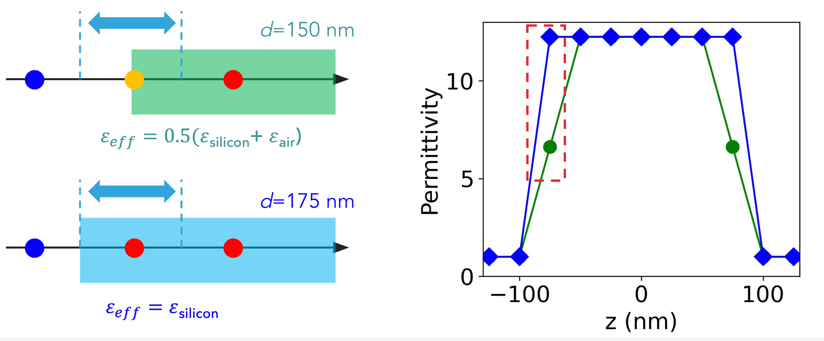
However, in this 1D case, this averaging is accurate because the dominant electric field is parallel to the dielectric grid points.
You can learn more about the subpixel averaging derivation from Maxwell’s equations in 1D in this lecture: Introduction to subpixel averaging.
2D & 3D Usage Caveats
In 2D, the subpixel averaging implementation depends on the polarization (\(s\) or \(p\)) of the incident electric field on the interface.
In 3D, the subpixel averaging is implemented with tensorial averaging due to arbitrary surface and field spatial orientations.
See also
- simulation_type#
- post_norm#
- internal_absorbers#
- plot_absorbers(x=None, y=None, z=None, hlim=None, vlim=None, alpha=None, ax=None, shifted=False)[source]#
Plot each of simulation’s port absorbers on a plane defined by one nonzero x,y,z coordinate.
- Parameters:
x (float = None) – position of plane in x direction, only one of x, y, z must be specified to define plane.
y (float = None) – position of plane in y direction, only one of x, y, z must be specified to define plane.
z (float = None) – position of plane in z direction, only one of x, y, z must be specified to define plane.
hlim (Tuple[float, float] = None) – The x range if plotting on xy or xz planes, y range if plotting on yz plane.
vlim (Tuple[float, float] = None) – The z range if plotting on xz or yz planes, y plane if plotting on xy plane.
alpha (float = None) – Opacity of the absorbers, If
Noneuses Tidy3d default.ax (matplotlib.axes._subplots.Axes = None) – Matplotlib axes to plot on, if not specified, one is created.
- Returns:
The supplied or created matplotlib axes.
- Return type:
matplotlib.axes._subplots.Axes
- plot(x=None, y=None, z=None, ax=None, source_alpha=None, monitor_alpha=None, lumped_element_alpha=None, absorber_alpha=None, absorber_actual_placement=False, hlim=None, vlim=None, fill_structures=True, **patch_kwargs)[source]#
Plot each of simulation’s components on a plane defined by one nonzero x,y,z coordinate.
- Parameters:
fill_structures (bool = True) – Whether to fill structures with color or just draw outlines.
x (float = None) – position of plane in x direction, only one of x, y, z must be specified to define plane.
y (float = None) – position of plane in y direction, only one of x, y, z must be specified to define plane.
z (float = None) – position of plane in z direction, only one of x, y, z must be specified to define plane.
source_alpha (float = None) – Opacity of the sources. If
None, uses Tidy3d default.monitor_alpha (float = None) – Opacity of the monitors. If
None, uses Tidy3d default.lumped_element_alpha (float = None) – Opacity of the lumped elements. If
None, uses Tidy3d default.absorber_alpha (float = None) – Opacity of the port absorbers. If
None, uses Tidy3d default.absorber_actual_placement (bool = False) – Use the exact placement of port absorbers which take into account their
shiftvalues.ax (matplotlib.axes._subplots.Axes = None) – Matplotlib axes to plot on, if not specified, one is created.
hlim (tuple[float, float] = None) – The x range if plotting on xy or xz planes, y range if plotting on yz plane.
vlim (tuple[float, float] = None) – The z range if plotting on xz or yz planes, y plane if plotting on xy plane.
- Returns:
The supplied or created matplotlib axes.
- Return type:
matplotlib.axes._subplots.Axes
See also
- plot_eps(x=None, y=None, z=None, freq=None, alpha=None, source_alpha=None, monitor_alpha=None, lumped_element_alpha=None, absorber_alpha=None, absorber_actual_placement=False, hlim=None, vlim=None, ax=None, eps_component=None, eps_lim=(None, None))[source]#
Plot each of simulation’s components on a plane defined by one nonzero x,y,z coordinate. The permittivity is plotted in grayscale based on its value at the specified frequency.
- Parameters:
x (float = None) – position of plane in x direction, only one of x, y, z must be specified to define plane.
y (float = None) – position of plane in y direction, only one of x, y, z must be specified to define plane.
z (float = None) – position of plane in z direction, only one of x, y, z must be specified to define plane.
freq (float = None) – Frequency to evaluate the relative permittivity of all mediums. If not specified, the central frequency of sources in the simulation will be used. If sources have different central frequencies, the relative permittivity will be evaluated at infinite frequency.
alpha (float = None) – Opacity of the structures being plotted. Defaults to the structure default alpha.
source_alpha (float = None) – Opacity of the sources. If
None, uses Tidy3d default.monitor_alpha (float = None) – Opacity of the monitors. If
None, uses Tidy3d default.lumped_element_alpha (float = None) – Opacity of the lumped elements. If
None, uses Tidy3d default.absorber_alpha (float = None) – Opacity of the port absorbers. If
None, uses Tidy3d default.absorber_actual_placement (bool = False) – Use the exact placement of port absorbers which take into account their
shiftvalues.ax (matplotlib.axes._subplots.Axes = None) – Matplotlib axes to plot on, if not specified, one is created.
hlim (tuple[float, float] = None) – The x range if plotting on xy or xz planes, y range if plotting on yz plane.
vlim (tuple[float, float] = None) – The z range if plotting on xz or yz planes, y plane if plotting on xy plane.
eps_component (Optional[PermittivityComponent] = None) – Component of the permittivity tensor to plot for anisotropic materials, e.g.
"xx","yy","zz","xy","yz", … Defaults toNone, which returns the average of the diagonal values.eps_lim (Tuple[float, float] = None) – Custom limits for eps coloring.
- Returns:
The supplied or created matplotlib axes.
- Return type:
matplotlib.axes._subplots.Axes
See also
- plot_structures_eps(x=None, y=None, z=None, freq=None, alpha=None, cbar=True, reverse=False, ax=None, hlim=None, vlim=None, eps_component=None, eps_lim=(None, None))[source]#
Plot each of simulation’s structures on a plane defined by one nonzero x,y,z coordinate. The permittivity is plotted in grayscale based on its value at the specified frequency.
- Parameters:
x (float = None) – position of plane in x direction, only one of x, y, z must be specified to define plane.
y (float = None) – position of plane in y direction, only one of x, y, z must be specified to define plane.
z (float = None) – position of plane in z direction, only one of x, y, z must be specified to define plane.
freq (float = None) – Frequency to evaluate the relative permittivity of all mediums. If not specified, the central frequency of sources in the simulation will be used. If sources have different central frequencies, the relative permittivity will be evaluated at infinite frequency.
reverse (bool = False) – If
False, the highest permittivity is plotted in black. IfTrue, it is plotteed in white (suitable for black backgrounds).cbar (bool = True) – Whether to plot a colorbar for the relative permittivity.
alpha (float = None) – Opacity of the structures being plotted. Defaults to the structure default alpha.
ax (matplotlib.axes._subplots.Axes = None) – Matplotlib axes to plot on, if not specified, one is created.
hlim (tuple[float, float] = None) – The x range if plotting on xy or xz planes, y range if plotting on yz plane.
vlim (tuple[float, float] = None) – The z range if plotting on xz or yz planes, y plane if plotting on xy plane.
eps_component (Optional[PermittivityComponent] = None) – Component of the permittivity tensor to plot for anisotropic materials, e.g.
"xx","yy","zz","xy","yz", … Defaults toNone, which returns the average of the diagonal values.eps_lim (Tuple[float, float] = None) – Custom limits for eps coloring.
- Returns:
The supplied or created matplotlib axes.
- Return type:
matplotlib.axes._subplots.Axes
- plot_pml(x=None, y=None, z=None, hlim=None, vlim=None, ax=None)[source]#
Plot each of simulation’s absorbing boundaries on a plane defined by one nonzero x,y,z coordinate.
- Parameters:
x (float = None) – position of plane in x direction, only one of x, y, z must be specified to define plane.
y (float = None) – position of plane in y direction, only one of x, y, z must be specified to define plane.
z (float = None) – position of plane in z direction, only one of x, y, z must be specified to define plane
hlim (tuple[float, float] = None) – The x range if plotting on xy or xz planes, y range if plotting on yz plane.
vlim (tuple[float, float] = None) – The z range if plotting on xz or yz planes, y plane if plotting on xy plane.
ax (matplotlib.axes._subplots.Axes = None) – Matplotlib axes to plot on, if not specified, one is created.
- Returns:
The supplied or created matplotlib axes.
- Return type:
matplotlib.axes._subplots.Axes
- property bounds_pml#
Simulation bounds including the PML regions.
- property simulation_bounds#
Simulation bounds including the PML regions.
- eps_bounds(freq=None)[source]#
Compute range of (real) permittivity present in the simulation at frequency “freq”.
- property pml_thicknesses#
Thicknesses (um) of absorbers in all three axes and directions (-, +)
- property internal_override_structures#
Internal mesh override structures. So far, internal override structures all come from layer_refinement_specs.
- Returns:
List of override structures.
- Return type:
list[MeshOverrideSructure]
- property internal_snapping_points#
Internal snapping points. So far, internal snapping points are generated by layer_refinement_specs.
- Returns:
List of snapping points coordinates.
- Return type:
list[CoordinateOptional]
- plot_lumped_elements(x=None, y=None, z=None, hlim=None, vlim=None, alpha=None, ax=None)[source]#
Plot each of simulation’s lumped elements on a plane defined by one nonzero x,y,z coordinate.
- Parameters:
x (float = None) – position of plane in x direction, only one of x, y, z must be specified to define plane.
y (float = None) – position of plane in y direction, only one of x, y, z must be specified to define plane.
z (float = None) – position of plane in z direction, only one of x, y, z must be specified to define plane.
hlim (tuple[float, float] = None) – The x range if plotting on xy or xz planes, y range if plotting on yz plane.
vlim (tuple[float, float] = None) – The z range if plotting on xz or yz planes, y plane if plotting on xy plane.
alpha (float = None) – Opacity of the lumped element, If
Noneuses Tidy3d default.ax (matplotlib.axes._subplots.Axes = None) – Matplotlib axes to plot on, if not specified, one is created.
- Returns:
The supplied or created matplotlib axes.
- Return type:
matplotlib.axes._subplots.Axes
- plot_grid(x=None, y=None, z=None, ax=None, hlim=None, vlim=None, override_structures_alpha=1, snapping_points_alpha=1, finest_grid_region_alpha=0.1, **kwargs)[source]#
Plot the cell boundaries as lines on a plane defined by one nonzero x,y,z coordinate.
- Parameters:
x (float = None) – position of plane in x direction, only one of x, y, z must be specified to define plane.
y (float = None) – position of plane in y direction, only one of x, y, z must be specified to define plane.
z (float = None) – position of plane in z direction, only one of x, y, z must be specified to define plane.
hlim (tuple[float, float] = None) – The x range if plotting on xy or xz planes, y range if plotting on yz plane.
vlim (tuple[float, float] = None) – The z range if plotting on xz or yz planes, y plane if plotting on xy plane.
override_structures_alpha (float = 1) – Opacity of the override structures.
snapping_points_alpha (float = 1) – Opacity of the snapping points.
finest_grid_region_alpha (float = 0.1) – Opacity of the shaded regions highlighting finest grid regions.
ax (matplotlib.axes._subplots.Axes = None) – Matplotlib axes to plot on, if not specified, one is created.
**kwargs – Optional keyword arguments passed to the matplotlib
LineCollection. For details on accepted values, refer to Matplotlib’s documentation.
- Returns:
The supplied or created matplotlib axes.
- Return type:
matplotlib.axes._subplots.Axes
- plot_boundaries(x=None, y=None, z=None, ax=None, **kwargs)[source]#
- Plot the simulation boundary conditions as lines on a plane
defined by one nonzero x,y,z coordinate.
- Parameters:
x (float = None) – position of plane in x direction, only one of x, y, z must be specified to define plane.
y (float = None) – position of plane in y direction, only one of x, y, z must be specified to define plane.
z (float = None) – position of plane in z direction, only one of x, y, z must be specified to define plane.
ax (matplotlib.axes._subplots.Axes = None) – Matplotlib axes to plot on, if not specified, one is created.
**kwargs –
Optional keyword arguments passed to the matplotlib
LineCollection. For details on accepted values, refer to Matplotlib’s documentation.
- Returns:
The supplied or created matplotlib axes.
- Return type:
matplotlib.axes._subplots.Axes
- property grid#
FDTD grid spatial locations and information.
- property static_structures#
Structures in simulation with all autograd tracers removed.
- property num_cells#
Number of cells in the simulation.
- Returns:
Number of yee cells in the simulation.
- Return type:
- property grid_info#
Dictionary collecting various properties of the grids in the simulation.
- property num_pml_layers#
Number of absorbing layers in all three axes and directions (-, +).
- discretize_monitor(monitor)[source]#
Grid on which monitor data corresponding to a given monitor will be computed.
- discretize(box, extend=False)[source]#
Grid containing only cells that intersect with a
Box.- Parameters:
box (
Box) – Rectangular geometry within simulation to discretize.extend (bool = False) – If
True, ensure that the returned indexes extend sufficiently in every direction to be able to interpolate any field component at any point within thebox, for field components sampled on the Yee grid.
- Returns:
The FDTD subgrid containing simulation points that intersect with
box.- Return type:
- epsilon(box, coord_key='centers', freq=None)[source]#
Get array of permittivity at volume specified by box and freq.
- Parameters:
box (
Box) – Rectangular geometry specifying where to measure the permittivity.coord_key (str = 'centers') – Specifies at what part of the grid to return the permittivity at. Accepted values are
{'centers', 'boundaries', 'Ex', 'Ey', 'Ez', 'Exy', 'Exz', 'Eyx',
'Eyz', 'Ezx', Ezy'}
. The field values (eg.'Ex') correspond to the corresponding field locations on the yee lattice. If field values are selected, the corresponding diagonal (eg.eps_xxin case of'Ex') or off-diagonal (eg.eps_xyin case of'Exy') epsilon component from the epsilon tensor is returned. Otherwise, the average of the main values is returned.freq (float = None) – The frequency to evaluate the mediums at. If not specified, evaluates at infinite frequency.
- Returns:
Datastructure containing the relative permittivity values and location coordinates. For details on xarray DataArray objects, refer to xarray’s Documentation.
- Return type:
Note
This method supports local subpixel averaging when the
tidy3d-extraspackage is installed. The behavior is controlled byconfig.simulation.use_local_subpixel. SeeSimulationConfig.use_local_subpixelfor details.See also
- Notebooks
- epsilon_on_grid(grid, coord_key='centers', freq=None)[source]#
Get array of permittivity at a given freq on a given grid.
- Parameters:
grid (
Grid) – Grid specifying where to measure the permittivity.coord_key (str = 'centers') – Specifies at what part of the grid to return the permittivity at. Accepted values are
{'centers', 'boundaries', 'Ex', 'Ey', 'Ez', 'Exy', 'Exz', 'Eyx',
'Eyz', 'Ezx', Ezy'}
. The field values (eg.'Ex') correspond to the corresponding field locations on the yee lattice. If field values are selected, the corresponding diagonal (eg.eps_xxin case of'Ex') or off-diagonal (eg.eps_xyin case of'Exy') epsilon component from the epsilon tensor is returned. Otherwise, the average of the main values is returned.freq (float = None) – The frequency to evaluate the mediums at. If not specified, evaluates at infinite frequency.
- Returns:
Datastructure containing the relative permittivity values and location coordinates. For details on xarray DataArray objects, refer to xarray’s Documentation.
- Return type:
Note
This method supports local subpixel averaging when the
tidy3d-extraspackage is installed. The behavior is controlled byconfig.simulation.use_local_subpixel. SeeSimulationConfig.use_local_subpixelfor details.
- property volumetric_structures#
Generate a tuple of structures wherein any 2D materials are converted to 3D volumetric equivalents.
- suggest_mesh_overrides(**kwargs)[source]#
Generate a
MeshOverrideStructureList which is automatically generated from structures in the simulation.
- subsection(region, boundary_spec=None, grid_spec=None, symmetry=None, warn_symmetry_expansion=True, sources=None, monitors=None, remove_outside_structures=True, remove_outside_grid_spec=False, remove_outside_custom_mediums=False, include_pml_cells=False, validate_geometries=True, deep_copy=True, internal_absorbers=None, **kwargs)[source]#
Generate a simulation instance containing only the
region.- Parameters:
region (
Box) – New simulation domain.boundary_spec (
BoundarySpec= None) – New boundary specification. IfNone, then it is inherited from the original simulation.grid_spec (
GridSpec= None) – New grid specification. IfNone, then it is inherited from the original simulation. Ifidentical, then the original grid is transferred directly as aCustomGrid. Note that in the latter case the region of the new simulation is snapped to the original grid lines.symmetry (tuple[Literal[0, -1, 1], Literal[0, -1, 1], Literal[0, -1, 1]] = None) – New simulation symmetry. If
None, then it is inherited from the original simulation. Note that in this case the size and placement of new simulation domain must be commensurate with the original symmetry.warn_symmetry_expansion (bool = True) – Whether to warn when the subsection is expanded to preserve symmetry.
sources (tuple[SourceType, ...] = None) – New list of sources. If
None, then the sources intersecting the new simulation domain are inherited from the original simulation.monitors (tuple[MonitorType, ...] = None) – New list of monitors. If
None, then the monitors intersecting the new simulation domain are inherited from the original simulation.remove_outside_structures (bool = True) – Remove structures outside of the new simulation domain.
remove_outside_grid_spec (bool = False) – Prune or clip
override_structures,layer_refinement_specs, andsnapping_pointsingrid_specto the requested region. Only applies when at least one axis usesAutoGridorQuasiUniformGrid.remove_outside_custom_mediums (bool = True) – Remove custom medium data outside of the new simulation domain.
include_pml_cells (bool = False) – Keep PML cells in simulation boundaries. Note that retained PML cells will be converted to regular cells, and the simulation domain boundary will be moved accordingly.
validate_geometries (bool = True) – If
False, skip validation for the geometries in the resulting simulation object. Simulation validators remain but only use the bounding box of the existing geometries. Used internally.deep_copy (bool = True) – Recursively copy all nested objects in the generated simulation object.
internal_absorbers (Tuple[InternalAbsorber, ...] = None) – New list of internal absorbers. If
None, then the absorbers intersecting the new simulation domain are inherited from the original simulation.**kwargs – Other arguments passed to new simulation instance.