Using the waveguide plugin to analyze waveguide modes

Using the waveguide plugin to analyze waveguide modes#

This notebook demonstrates the use of the waveguide plugin to quickly set-up waveguide simulations from usual geometries.

[1]:

from __future__ import annotations

import numpy as np
import tidy3d as td
import tidy3d.web as web
from matplotlib import pyplot
from tidy3d.plugins import waveguide

[2]:

# Media used in the examples
si = td.material_library["cSi"]["Li1993_293K"]
sio2 = td.material_library["SiO2"]["Horiba"]

Strip and Rib Geometries#

The class RectangularDielectric allows the creation of a variety of dielectric waveguide geometries common in integrated photonics.

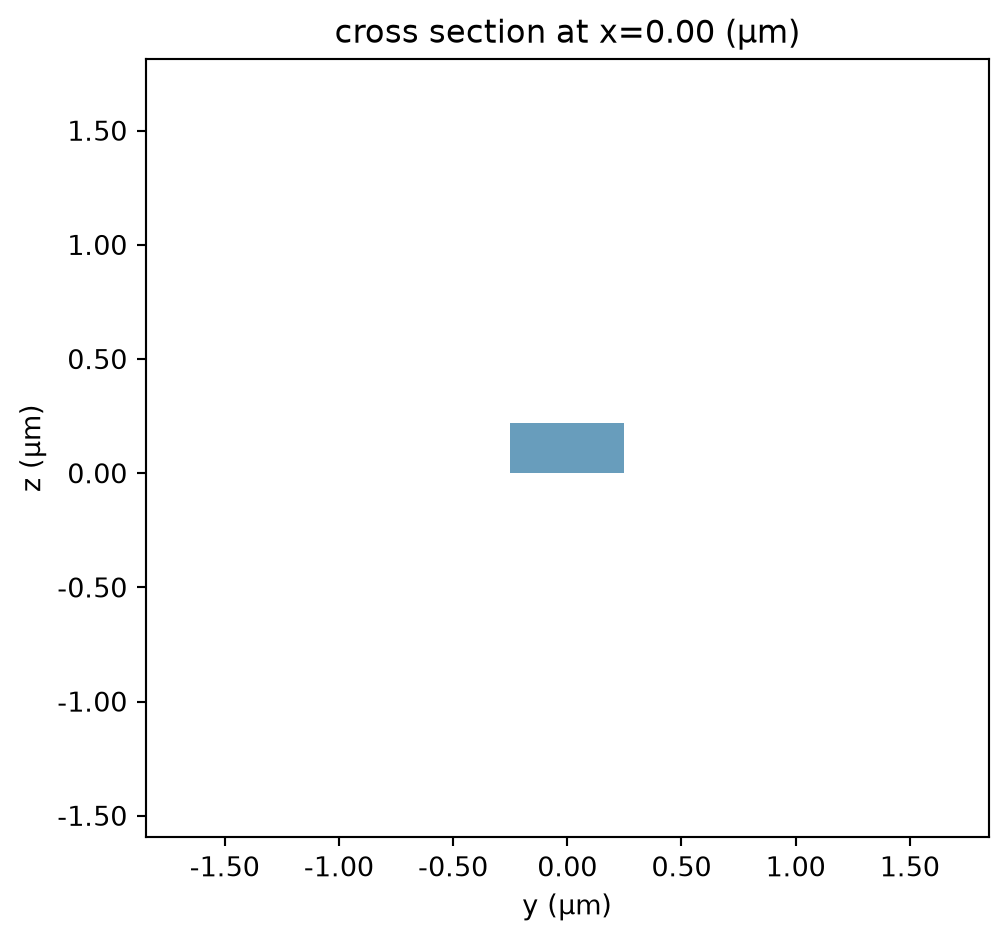
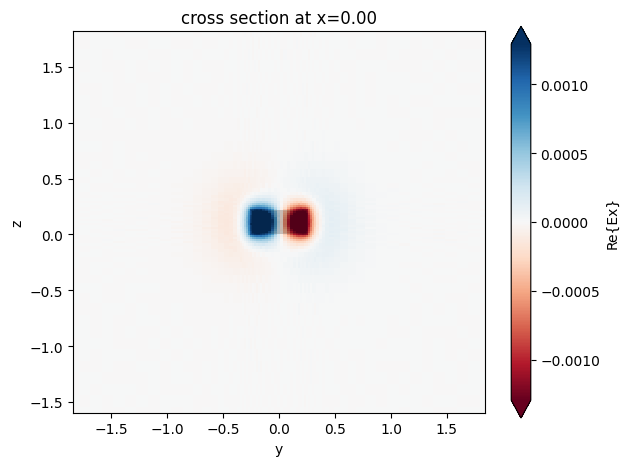
First we take a look at a strip silicon waveguide and plot the fundamental quasi-TE and quasi-TM modes, along with their effective indices:

[3]:

strip = waveguide.RectangularDielectric(
    wavelength=1.55,
    core_width=0.5,
    core_thickness=0.22,
    core_medium=si,
    clad_medium=sio2,
    mode_spec=td.ModeSpec(num_modes=2, group_index_step=True),
)

# Take a look at the waveguide cross-section
_ = strip.plot_structures(x=0)

../_images/notebooks_WaveguidePluginDemonstration_4_0.png

[4]:

strip.plot_field("Ex", mode_index=0)

../_images/notebooks_WaveguidePluginDemonstration_5_0.png

[5]:

# Mode data
print(f"Effective indices: {strip.n_eff.values}")
print(f"Effective mode areas (µm²): {strip.mode_area.values}")
print(f"Group index: {strip.n_group.values}")

fig, ax = pyplot.subplots(1, 2, figsize=(10, 4), tight_layout=True)

# quasi-TE mode
strip.plot_field("Ey", mode_index=0, ax=ax[0])

# quasi-TM mode
strip.plot_field("Ez", mode_index=1, ax=ax[1])

Effective indices: [[2.44624476 1.7895686 ]]
Effective mode areas (µm²): [[0.19145485 0.35608204]]
Group index: [[4.17353874 3.73989668]]

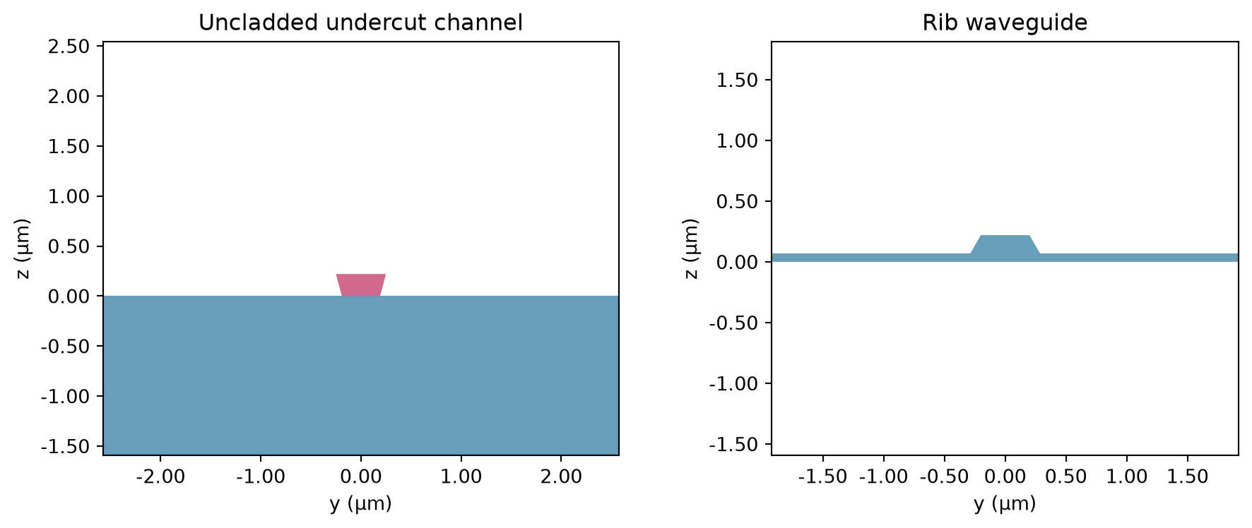
../_images/notebooks_WaveguidePluginDemonstration_6_1.png

It is possible to define waveguides with different substrate and cladding, angled sidewalls, and rib geometry:

[6]:

fig, ax = pyplot.subplots(1, 2, figsize=(10, 4), tight_layout=True)

undercut = strip = waveguide.RectangularDielectric(
    wavelength=1.55,
    core_width=0.5,
    core_thickness=0.22,
    sidewall_angle=-np.pi / 12,
    core_medium=si,
    clad_medium=td.Medium(permittivity=1.0),
    box_medium=sio2,
)

undercut.plot_structures(x=0, ax=ax[0])
_ = ax[0].set_title("Uncladded undercut channel")

rib = strip = waveguide.RectangularDielectric(
    wavelength=1.55,
    core_width=0.4,
    core_thickness=0.22,
    slab_thickness=0.07,
    sidewall_angle=np.pi / 6,
    core_medium=si,
    clad_medium=sio2,
)

rib.plot_structures(x=0, ax=ax[1])
_ = ax[1].set_title("Rib waveguide")

../_images/notebooks_WaveguidePluginDemonstration_8_0.png

FDTD Simulation#

The waveguide structures can be used in Tidy3D simulations as conventional structures. The origin, length, and orientation of the waveguides can be selected at creation to fit the most common simulation configurations.

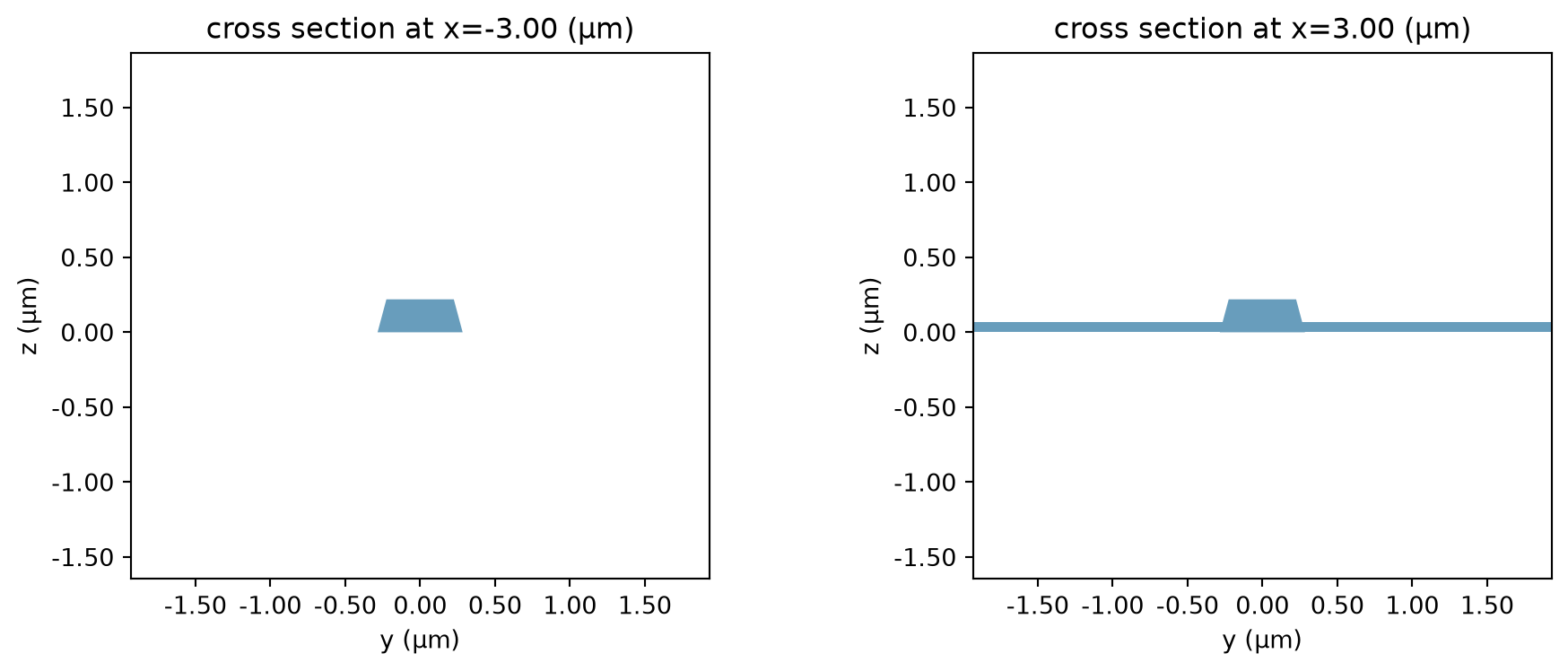
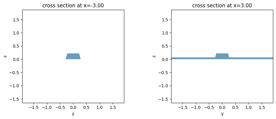
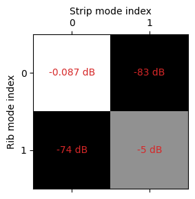
In the following example, we simulate the effect of directly coupling strip and rib geometries without any tapering and compare the result with the modal overlap calculation between the two modes.

[7]:

length = 6.0

strip, rib = (
    waveguide.RectangularDielectric(
        wavelength=np.linspace(1.5, 1.6, 11),
        core_width=0.45,
        core_thickness=0.22,
        core_medium=si,
        clad_medium=sio2,
        slab_thickness=0.07 if slab else 0,
        length=length,
        origin=(0.5 * length if slab else -0.5 * length, 0, 0),
        sidewall_angle=np.pi / 12,
    )
    for slab in (False, True)
)

fig, ax = pyplot.subplots(1, 2, figsize=(10, 4), tight_layout=True)
strip.plot_structures(x=-0.5 * length, ax=ax[0])
rib.plot_structures(x=0.5 * length, ax=ax[1])

pyplot.show()

../_images/notebooks_WaveguidePluginDemonstration_10_0.png

[8]:

# Calculate the mode overlap between waveguides
overlap = strip.mode_solver.data.outer_dot(rib.mode_solver.data, False)

# Show the overlap at the central frequency
f = strip.mode_solver.freqs[strip.wavelength.size // 2]

fig, ax = pyplot.subplots(1, 1, figsize=(3, 3), tight_layout=True)

ax.matshow(np.abs(overlap.sel(f=f).values), cmap="gray")
ax.grid(False)

for mi0 in overlap.coords["mode_index_0"]:
    for mi1 in overlap.coords["mode_index_1"]:
        ovl_dB = 20 * np.log10(np.abs(overlap.sel(f=f, mode_index_0=mi0, mode_index_1=mi1).item()))
        ax.text(mi0, mi1, f"{ovl_dB:.2g} dB", ha="center", va="center", color="tab:red")

ax.set_ylabel("Rib mode index")
ax.set_xlabel("Strip mode index")
ax.xaxis.set_label_position("top")

../_images/notebooks_WaveguidePluginDemonstration_11_0.png

[9]:

freqs = strip.mode_solver.freqs
source_time = td.GaussianPulse(freq0=0.5 * (freqs[0] + freqs[-1]), fwidth=abs(freqs[0] - freqs[-1]))

src_gap = 0.5
mode_src = td.ModeSource(
    center=(-0.5 * length - src_gap / 2, 0, 0),
    size=(0, td.inf, td.inf),
    source_time=source_time,
    num_freqs=5,
    direction="+",
    mode_spec=strip.mode_spec,
    mode_index=0,
)

strip_mnt = strip.mode_solver.to_monitor(freqs=freqs, name="strip")

rib_mnt = rib.mode_solver.to_monitor(freqs=freqs, name="rib")

field_mnt = td.FieldMonitor(
    center=(0, 0, 0.5 * strip.core_thickness),
    size=(td.inf, td.inf, 0),
    freqs=freqs,
    name="field",
)

sim_size = (length + 2 * src_gap, strip.width, strip.height)
sim_center = (0, 0, strip.mode_solver.plane.center[2])

sim = td.Simulation(
    size=sim_size,
    center=sim_center,
    grid_spec=td.GridSpec.auto(min_steps_per_wvl=20),
    structures=strip.structures + rib.structures,
    sources=[mode_src],
    monitors=[strip_mnt, rib_mnt, field_mnt],
    run_time=1e-12,
    boundary_spec=td.BoundarySpec.all_sides(boundary=td.PML()),
)

fig, ax = pyplot.subplots(2, 2, figsize=(11, 10), tight_layout=True)
sim.plot(z=0.5 * strip.core_thickness, ax=ax[0, 0])
sim.plot(z=0.5 * rib.slab_thickness, ax=ax[0, 1])
sim.plot(x=-0.5 * length, ax=ax[1, 0])
sim.plot(x=0.5 * length, ax=ax[1, 1])
pyplot.show()

../_images/notebooks_WaveguidePluginDemonstration_12_0.png

[10]:

# Run the simulation and download the resulting data
data = web.run(sim, task_name="untapered", verbose=True)

15:35:41 UTC Created task 'untapered' with resource_id
             'fdve-19703474-073d-4e7a-844b-af5b6690315f' and task_type 'FDTD'.

             View task using web UI at
             'https://tidy3d.simulation.cloud/workbench?taskId=fdve-19703474-073
             d-4e7a-844b-af5b6690315f'.

             Task folder: 'default'.

15:35:43 UTC Estimated FlexCredit cost: 0.123. This assumes the FDTD solver runs
             for the full simulation time; if early shutoff is reached, the
             billed cost can be lower. Use 'web.real_cost(task_id)' to get the
             billed FlexCredit cost after a simulation run.

             status = queued

             To cancel the simulation, use 'web.abort(task_id)' or
             'web.delete(task_id)' or abort/delete the task in the web UI.
             Terminating the Python script will not stop the job running on the
             cloud.

15:35:53 UTC status = preprocess

15:36:02 UTC starting up solver

15:36:03 UTC running solver

15:36:15 UTC early shutoff detected at 20%, exiting.

15:36:16 UTC status = postprocess

15:36:21 UTC status = success

15:36:23 UTC View simulation result at
             'https://tidy3d.simulation.cloud/workbench?taskId=fdve-19703474-073
             d-4e7a-844b-af5b6690315f'.

15:36:26 UTC Loading results from simulation_data.hdf5

[11]:

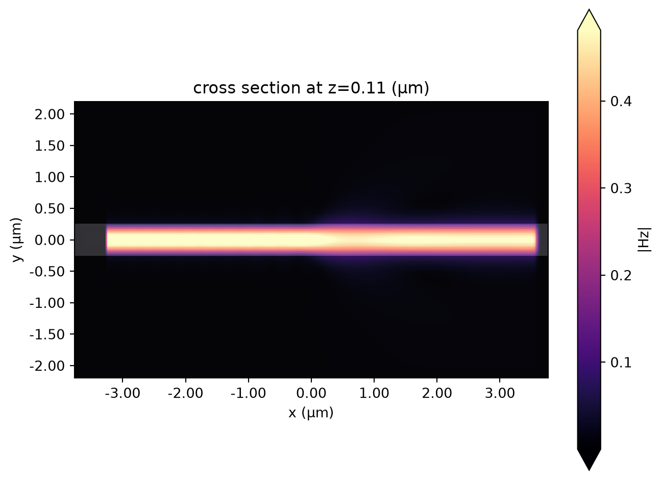
_ = data.plot_field("field", "Hz", val="abs", f=f)

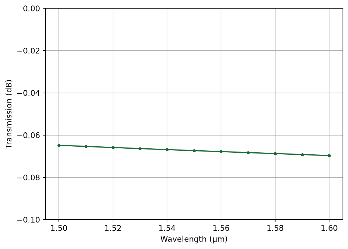
../_images/notebooks_WaveguidePluginDemonstration_14_0.png

Looking at the power transmission, we see almost the same result as obtained from the overlap calculation:

[12]:

rib_transmission = data["rib"].amps.sel(direction="+", mode_index=0)
fig, ax = pyplot.subplots(1, 1)
ax.plot(rib.wavelength, 20 * np.log10(np.abs(rib_transmission.values)), ".-")
ax.set(
    xlabel="Wavelength (μm)",
    ylabel="Transmission (dB)",
    ylim=(-0.1, 0),
)
ax.grid()

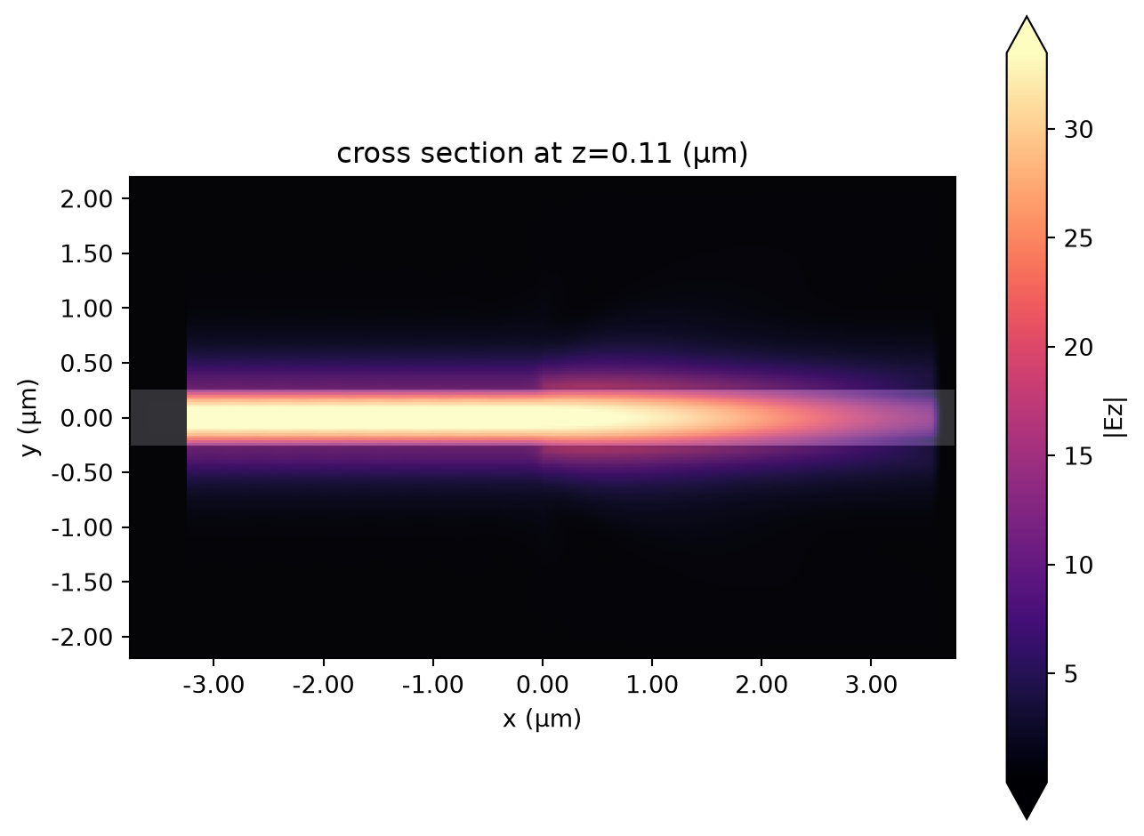
../_images/notebooks_WaveguidePluginDemonstration_16_0.png

We can look at the first quasi-TM mode as well:

[13]:

# mode_src_tm = mode_src.copy(update={"mode_index": 1})
mode_src_tm = td.ModeSource(
    center=(-0.5 * length - src_gap / 2, 0, 0),
    size=(0, td.inf, td.inf),
    source_time=source_time,
    num_freqs=5,
    direction="+",
    mode_spec=strip.mode_spec,
    mode_index=1,
)

sim_tm = sim.copy(update={"sources": [mode_src_tm]})
data_tm = td.web.run(sim_tm, task_name="untapered_tm", verbose=True)
_ = data_tm.plot_field("field", "Ez", val="abs", f=f)

15:36:27 UTC Created task 'untapered_tm' with resource_id
             'fdve-d10c1d11-1b46-439f-9af4-8191ecf11fbe' and task_type 'FDTD'.

             View task using web UI at
             'https://tidy3d.simulation.cloud/workbench?taskId=fdve-d10c1d11-1b4
             6-439f-9af4-8191ecf11fbe'.

             Task folder: 'default'.

15:36:29 UTC Estimated FlexCredit cost: 0.123. This assumes the FDTD solver runs
             for the full simulation time; if early shutoff is reached, the
             billed cost can be lower. Use 'web.real_cost(task_id)' to get the
             billed FlexCredit cost after a simulation run.

             status = queued

             To cancel the simulation, use 'web.abort(task_id)' or
             'web.delete(task_id)' or abort/delete the task in the web UI.
             Terminating the Python script will not stop the job running on the
             cloud.

15:36:41 UTC status = preprocess

15:36:48 UTC starting up solver

             running solver

15:37:03 UTC early shutoff detected at 20%, exiting.

             status = postprocess

15:37:06 UTC status = success

15:37:08 UTC View simulation result at
             'https://tidy3d.simulation.cloud/workbench?taskId=fdve-d10c1d11-1b4
             6-439f-9af4-8191ecf11fbe'.

15:37:11 UTC Loading results from simulation_data.hdf5

../_images/notebooks_WaveguidePluginDemonstration_18_24.png

[14]:

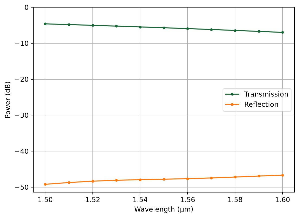
rib_transmission = data_tm["rib"].amps.sel(direction="+", mode_index=1)
strip_reflection = data_tm["strip"].amps.sel(direction="-", mode_index=1)

fig, ax = pyplot.subplots(1, 1)
ax.plot(rib.wavelength, 20 * np.log10(np.abs(rib_transmission.values)), ".-", label="Transmission")
ax.plot(rib.wavelength, 20 * np.log10(np.abs(strip_reflection.values)), ".-", label="Reflection")
ax.set(
    xlabel="Wavelength (μm)",
    ylabel="Power (dB)",
    ylim=(None, 0),
)
ax.legend()
ax.grid()

../_images/notebooks_WaveguidePluginDemonstration_19_0.png

A Note about Accuracy#

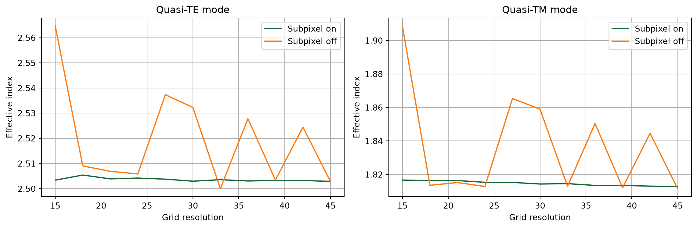
By default, the waveguide class uses grid_resolution = 15. This value is enough for quick mode solving with effective indices relatively accurate (usually within 10% of the best estimate). If higher accuracy is desired, grid_resolution can be increased to higher values, for example, to improve the calculation of derived values (group index, coupling length, mode losses, etc.).

Another important factor for accuracy is subpixel averaging, which smooths the material interfaces on the Yee grid and greatly improves the convergence of the effective indices with respect to grid resolution. The mode solver applies subpixel averaging automatically when the tidy3d-extras package is installed (pip install "tidy3d[extras]"), with the whole calculation running locally. Alternatively, the mode solver can also be run in the cloud with web.run(wg.mode_solver, task_name="mode_solver"), in which case subpixel averaging is applied as well.

To see the effect of subpixel averaging, we can disable it by setting td.config.simulation.use_local_subpixel = False. Below we compare the effective indices calculated with and without subpixel averaging as a function of grid resolution:

[15]:

wg_base = waveguide.RectangularDielectric(
    wavelength=1.55,
    core_width=0.5,
    core_thickness=0.22,
    core_medium=si,
    clad_medium=sio2,
    sidewall_angle=np.pi / 18,
)

grid_resolution = np.arange(15, 46, 3)
n_eff = ([], [])

for res in grid_resolution:
    print("Solving for resolution =", res, flush=True)
    td.config.simulation.use_local_subpixel = True
    wg = wg_base.copy(update={"grid_resolution": int(res)})
    n_eff[0].append(wg.n_eff.values)
    td.config.simulation.use_local_subpixel = False
    wg = wg_base.copy(update={"grid_resolution": int(res)})
    n_eff[1].append(wg.n_eff.values)

# restore subpixel averaging
td.config.simulation.use_local_subpixel = True

n_eff = [np.squeeze(n) for n in n_eff]

Solving for resolution = 15
Solving for resolution = 18
Solving for resolution = 21
Solving for resolution = 24
Solving for resolution = 27
Solving for resolution = 30
Solving for resolution = 33
Solving for resolution = 36
Solving for resolution = 39
Solving for resolution = 42
Solving for resolution = 45

[16]:

_, ax = pyplot.subplots(1, 2, tight_layout=True, figsize=(12, 4))

for i in range(2):
    ax[i].plot(grid_resolution, n_eff[0][:, i], label="Subpixel on")
    ax[i].plot(grid_resolution, n_eff[1][:, i], label="Subpixel off")
    ax[i].legend()
    ax[i].set(xlabel="Grid resolution", ylabel="Effective index")
    ax[i].grid()

ax[0].set_title("Quasi-TE mode")
ax[1].set_title("Quasi-TM mode")
pyplot.show()

../_images/notebooks_WaveguidePluginDemonstration_22_0.png

Waveguide Bends#

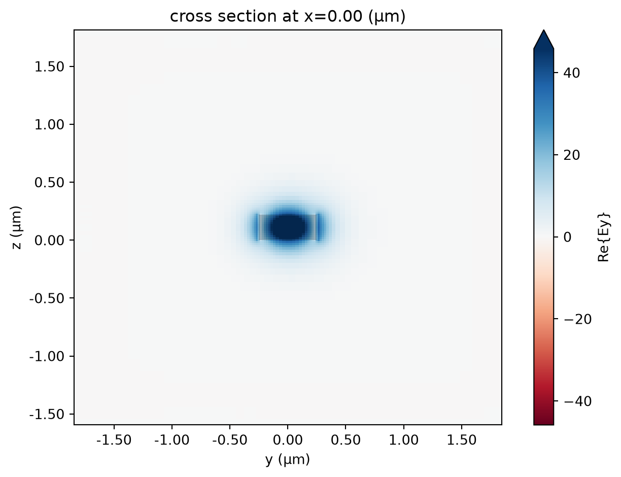
Waveguide bends can be modeled by setting the appropriate attributes in the mode specification.

[17]:

bend = waveguide.RectangularDielectric(
    wavelength=1.55,
    core_width=0.5,
    core_thickness=0.22,
    core_medium=si,
    clad_medium=sio2,
    mode_spec=td.ModeSpec(
        num_modes=1,
        bend_radius=5,
        bend_axis=1,
        num_pml=(12, 12),
    ),
)

fig, ax = pyplot.subplots(1, 1, tight_layout=True)
bend.plot_field("Ey", mode_index=0, ax=ax)

print(f"Complex effective index: {bend.n_complex.item():g}")

Complex effective index: 2.44394+5.30488e-05j

../_images/notebooks_WaveguidePluginDemonstration_24_1.png

Let’s create a helper function to convert the imaginary part of the complex effective index into loss in dB/cm:

[18]:

def loss_dB_per_cm(n_complex):
    alpha = 2 * np.pi * n_complex.imag * n_complex.f / td.C_0  # µm⁻¹
    return 1e4 * 20 * np.log10(np.e) * alpha  # dB/cm


print(f"Curvature loss: {loss_dB_per_cm(bend.n_complex).item():.1f} dB/cm")

Curvature loss: 18.7 dB/cm

We can put it all together to plot loss as a function of bend radius.

[19]:

radii = 5 * 10 ** np.linspace(0, 1, 10)
bend_data = []
for radius in radii:
    print(f"Solving for radius = {radius:.2f}", flush=True)
    bend = waveguide.RectangularDielectric(
        wavelength=1.55,
        core_width=0.5,
        core_thickness=0.22,
        core_medium=si,
        clad_medium=sio2,
        mode_spec=td.ModeSpec(
            num_modes=2,
            bend_radius=radius,
            bend_axis=1,
            num_pml=(12, 12),
        ),
    )
    bend_data.append(bend.mode_solver.data)

Solving for radius = 5.00

15:38:19 UTC WARNING: Mode field at frequency index 0, mode index 1 does not    
             decay at the plane boundaries.

Solving for radius = 6.46

15:38:23 UTC WARNING: Mode field at frequency index 0, mode index 1 does not    
             decay at the plane boundaries.

Solving for radius = 8.34
Solving for radius = 10.77
Solving for radius = 13.91
Solving for radius = 17.97
Solving for radius = 23.21
Solving for radius = 29.97
Solving for radius = 38.71
Solving for radius = 50.00

[20]:

fig, ax = pyplot.subplots(1, 2, figsize=(11, 4), tight_layout=True)

ax[0].plot(radii, [data.n_eff.isel(mode_index=0).item() for data in bend_data], ".-")
ax[0].set_xlabel("Bend radius (μm)")
ax[0].set_ylabel("Effective index")
ax[0].grid()

ax[1].plot(
    radii, [loss_dB_per_cm(data.n_complex).isel(mode_index=0).item() for data in bend_data], ".-"
)
ax[1].set_xlabel("Bend radius (μm)")
ax[1].set_ylabel("Curvature loss (dB/cm)")
ax[1].grid()

../_images/notebooks_WaveguidePluginDemonstration_29_0.png

Coupled Waveguides#

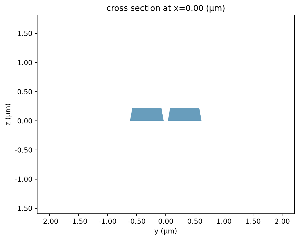
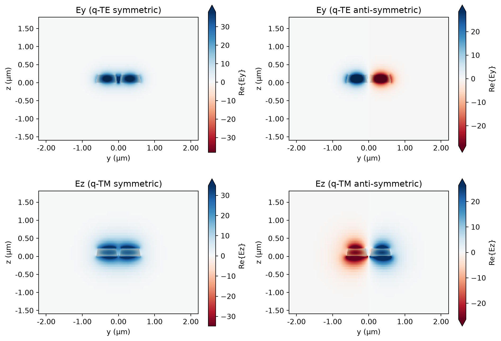
The RectangularDielectric class supports modeling coupled waveguides by passing an array of core widths (and a corresponding array of gaps between adjacent cores).

[21]:

coupled = waveguide.RectangularDielectric(
    wavelength=1.55,
    core_width=(0.5, 0.5),
    core_thickness=0.22,
    core_medium=si,
    clad_medium=sio2,
    gap=0.15,
    sidewall_angle=np.pi / 18,
    mode_spec=td.ModeSpec(num_modes=4),
)

_ = coupled.plot_structures(x=0)

../_images/notebooks_WaveguidePluginDemonstration_31_0.png

[22]:

# Mode data
print(f"Effective indices: {coupled.n_eff.values}")
print(f"Effective mode areas (µm²): {coupled.mode_area.values}")

fig, ax = pyplot.subplots(2, 2, figsize=(10, 7), tight_layout=True)

coupled.plot_field("Ey", mode_index=0, ax=ax[0, 0])
ax[0, 0].set_title("Ey (q-TE symmetric)")

coupled.plot_field("Ey", mode_index=1, ax=ax[0, 1])
ax[0, 1].set_title("Ey (q-TE anti-symmetric)")

coupled.plot_field("Ez", mode_index=2, ax=ax[1, 0])
ax[1, 0].set_title("Ez (q-TM symmetric)")

coupled.plot_field("Ez", mode_index=3, ax=ax[1, 1])
ax[1, 1].set_title("Ez (q-TM anti-symmetric)")

pyplot.show()

Effective indices: [[2.52944789 2.48996313 1.89128153 1.76011906]]
Effective mode areas (µm²): [[0.3678233  0.35555273 0.67381531 0.63189799]]

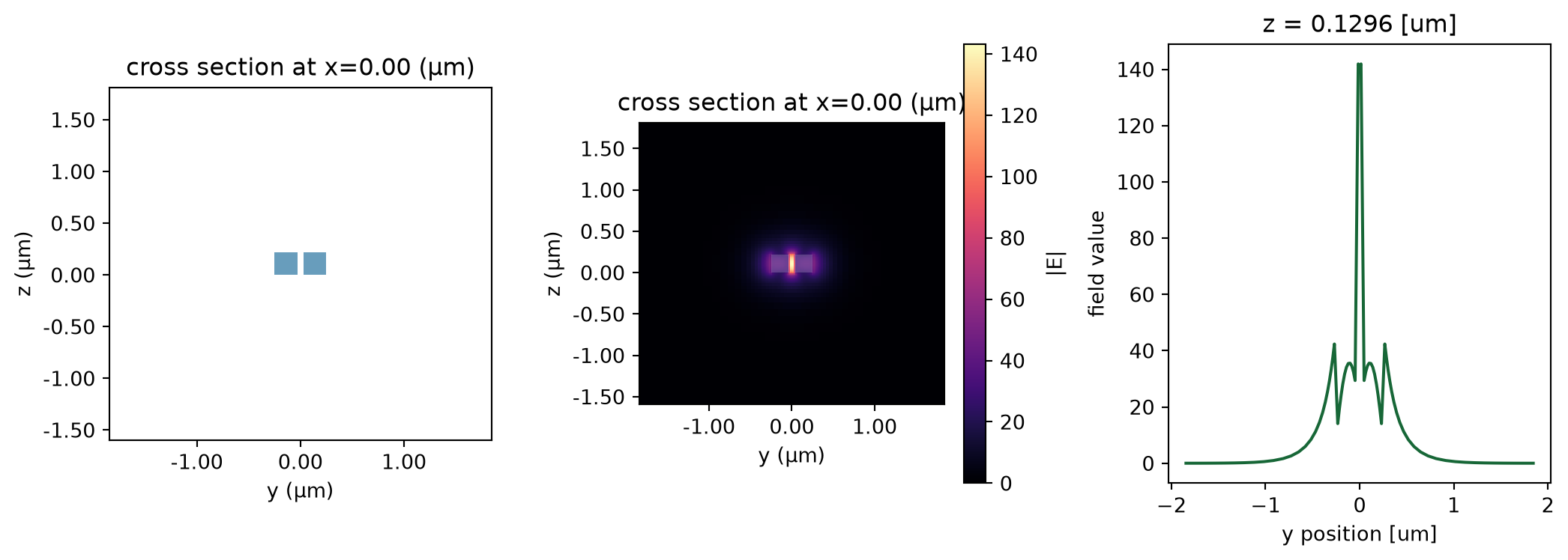
../_images/notebooks_WaveguidePluginDemonstration_32_1.png

In a similar fashion, vertical slot waveguides can also be simulated easily:

[23]:

slot = waveguide.RectangularDielectric(
    wavelength=1.55,
    core_width=(0.22, 0.22),
    core_thickness=0.22,
    core_medium=si,
    clad_medium=sio2,
    gap=0.06,
    mode_spec=td.ModeSpec(num_modes=1),
)

fig, ax = pyplot.subplots(1, 3, figsize=(11, 4), tight_layout=True)

slot.plot_structures(x=0, ax=ax[0])

# We use 'robust=False' because we're interested in the large values at the slot
slot.plot_field("E", val="abs", ax=ax[1], robust=False)

# Plot a cross-section of the field component normal to the gap
ey = slot.mode_solver.data.Ey
_ = ey.squeeze(drop=True).sel(z=0.55 * slot.core_thickness, method="nearest").real.plot(ax=ax[2])

../_images/notebooks_WaveguidePluginDemonstration_34_0.png

Surface Models#

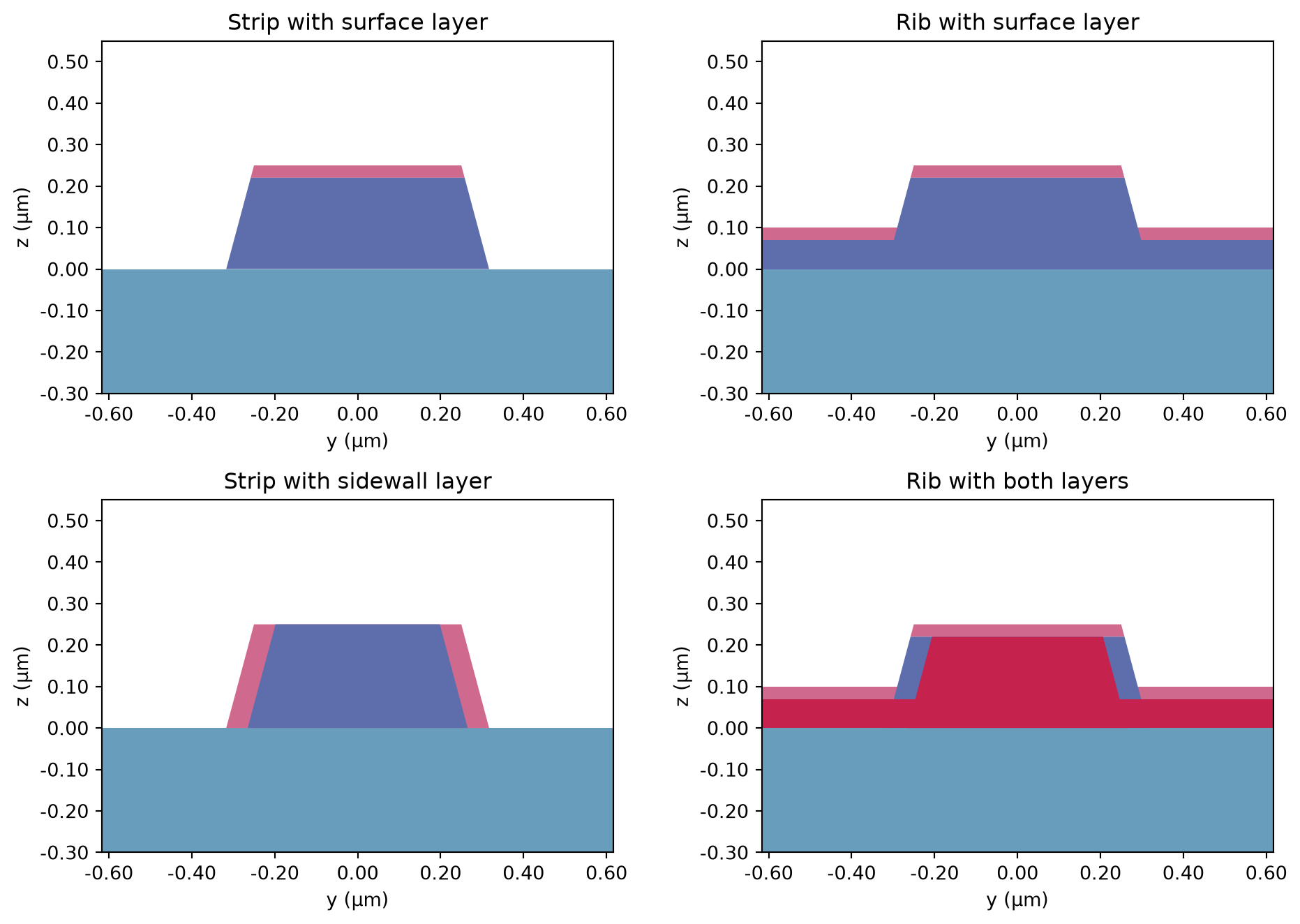
Besides using lossy materials for all waveguide regions (core, and upper and lower claddings), it is also possible to create separate medium layers along the sidewalls and top surfaces of the waveguide to model localized losses independently.

In the following models, we exaggerate those regions and decrease the domain size only to show a close-up of the resulting geometry. Decreasing the domain size is only advisable if we know the modes will have properly decayed to insignificant values at the domain boundaries. Also note that the colors in each plot correspond to different materials.

[24]:

fig, ax = pyplot.subplots(2, 2, figsize=(10, 7), tight_layout=True)

lossy0 = waveguide.RectangularDielectric(
    wavelength=1.55,
    core_width=0.5,
    core_thickness=0.25,
    core_medium=si,
    box_medium=sio2,
    clad_medium=td.Medium(permittivity=1.0),
    gap=0.15,
    sidewall_angle=np.pi / 12,
    surface_thickness=0.03,
    surface_medium=td.Medium.from_nk(n=3.4, k=0.008, freq=td.C_0 / 1.55),
    side_margin=0.3,
    clad_thickness=0.3,
    box_thickness=0.3,
)

lossy0.plot_structures(x=0, ax=ax[0, 0])
ax[0, 0].set_title("Strip with surface layer")

lossy1 = waveguide.RectangularDielectric(
    wavelength=1.55,
    core_width=0.5,
    core_thickness=0.25,
    slab_thickness=0.1,
    core_medium=si,
    box_medium=sio2,
    clad_medium=td.Medium(permittivity=1.0),
    gap=0.15,
    sidewall_angle=np.pi / 12,
    surface_thickness=0.03,
    surface_medium=td.Medium.from_nk(n=3.4, k=0.008, freq=td.C_0 / 1.55),
    side_margin=0.3,
    clad_thickness=0.3,
    box_thickness=0.3,
)

lossy1.plot_structures(x=0, ax=ax[0, 1])
ax[0, 1].set_title("Rib with surface layer")

lossy2 = waveguide.RectangularDielectric(
    wavelength=1.55,
    core_width=0.5,
    core_thickness=0.25,
    core_medium=si,
    box_medium=sio2,
    clad_medium=td.Medium(permittivity=1.0),
    gap=0.15,
    sidewall_angle=np.pi / 12,
    sidewall_thickness=0.05,
    sidewall_medium=td.Medium.from_nk(n=3.2, k=0.01, freq=td.C_0 / 1.55),
    side_margin=0.3,
    clad_thickness=0.3,
    box_thickness=0.3,
)

lossy2.plot_structures(x=0, ax=ax[1, 0])
ax[1, 0].set_title("Strip with sidewall layer")

lossy3 = waveguide.RectangularDielectric(
    wavelength=1.55,
    core_width=0.5,
    core_thickness=0.25,
    slab_thickness=0.1,
    core_medium=si,
    box_medium=sio2,
    clad_medium=td.Medium(permittivity=1.0),
    gap=0.15,
    sidewall_angle=np.pi / 12,
    sidewall_thickness=0.05,
    sidewall_medium=td.Medium.from_nk(n=3.2, k=0.01, freq=td.C_0 / 1.55),
    surface_thickness=0.03,
    surface_medium=td.Medium.from_nk(n=3.4, k=0.008, freq=td.C_0 / 1.55),
    side_margin=0.3,
    clad_thickness=0.3,
    box_thickness=0.3,
)

lossy3.plot_structures(x=0, ax=ax[1, 1])
_ = ax[1, 1].set_title("Rib with both layers")

../_images/notebooks_WaveguidePluginDemonstration_36_0.png