Thermally tuned waveguide#
In this example we use Tidy3D’s heat solver to investigate tuning of a straight rectangular waveguide using a heating strip.
[1]:
import numpy as np
import tidy3d as td
import tidy3d.web as web
from matplotlib import pyplot as plt
Note that package vtk is required to use full visualization capabilities of heat solver data. To install a compatible version of vtk one can use pip install tidy3d[vtk] command.
[2]:
wvl_um = 1.55
freq0 = td.C_0 / wvl_um
Setup Simulation Scene#
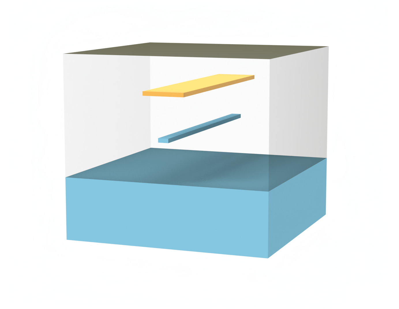
The simulation setup consists of a silicon waveguide in a silicon dioxide cladding on top of a silicon wafer. The heating strip is placed in the cladding above the waveguide. Let us define basic geometric parameters of simulated structures.
[3]:
# in um

w_sim = 16  # simulation width
h_buffer = 1  # vertical simulation buffer

h_clad = 2.8  # thickness of cladding
h_box = 2  # thickness of buried oxide
h_wafer = 0.5  # wafer thickness

# waveguide parameters
w_core = 0.5
h_core = 0.22

# heater parameters
h_heater = 0.14
w_heater = 2
d_heater = 2  # distance between heater and waveguide
We will place the wafer’s top surface at location \(z=0\). Let us define vertical locations of each structure. Note that we will model buried oxide and cladding as a single structure since they are made of the same material.
[4]:
z_wafer = -h_wafer / 2
z_core = h_box + h_core / 2
z_heater = h_box + h_core + d_heater + h_heater / 2

box_clad_max = h_box + h_clad
box_clad_min = (
    -h_wafer / 2
)  # make structures overlap to ensure no gaps due to numerical roundoff errors
h_box_clad = box_clad_max - box_clad_min
z_box_clad = (box_clad_max + box_clad_min) / 2

z_sim = (h_box + h_clad - h_wafer) / 2
h_sim = h_box + h_clad + h_wafer + 2 * h_buffer
Define optic and thermal properties of materials.
[5]:
Si_n = 3.4777  # Si refraction index
Si_n_slope = 1.86e-4  # Si thermo-optic coefficient dn/dT, 1/K
Si_k = 148e-6  # Si thermal conductivity, W / (um * K)
Si_s = 710  # Si specific heat capacity, J / (Kg * K)

SiO2_n = 1.444  # SiO2 refraction index
SiO2_n_slope = 1e-5  # SiO2 thermo-optic coefficient dn/dT, 1/K
SiO2_k = 1.38e-6  # SiO2 thermal conductivity, W/(um*K)
SiO2_s = 709  # SiO2 specific heat capacity, J / (Kg * K)

TiN_k = 28e-6  # TiN thermal conductivity W/(um*K)
TiN_s = 598  # TiN specific heat capacity, J / (Kg * K)
TiN_sigma = 2.3  # Electric conductivity of TiN, S/um
Create material classes containing relevant information for each medium. Note that we use class PerturbationMedium to specify sensitivity of optic properties to temperature and field heat_spec to specify thermal properties. Optic characteristics of the heating strip material is modeled as a perfect electric conductor.
[6]:
Si = td.PerturbationMedium.from_unperturbed(
    medium=td.Medium.from_nk(n=Si_n, k=0, freq=freq0),
    perturbation_spec=td.IndexPerturbation(
        delta_n=td.ParameterPerturbation(
            heat=td.LinearHeatPerturbation(coeff=Si_n_slope, temperature_ref=300)
        ),
        freq=freq0,
    ),
    heat_spec=td.SolidSpec(
        conductivity=Si_k,
        capacity=Si_s,
    ),
    name="Si",
)

# an alternative but equivalent way of defining a medium specification
SiO2 = td.PerturbationMedium(
    permittivity=SiO2_n**2,
    perturbation_spec=td.IndexPerturbation(
        delta_n=td.ParameterPerturbation(
            heat=td.LinearHeatPerturbation(coeff=SiO2_n_slope, temperature_ref=300)
        ),
        freq=freq0,
    ),
    heat_spec=td.SolidSpec(
        conductivity=SiO2_k,
        capacity=SiO2_s,
    ),
    name="SiO2",
)

TiN = td.PECMedium(
    heat_spec=td.SolidSpec(
        conductivity=TiN_k,
        capacity=TiN_s,
    ),
    name="TiN",
)

air = td.Medium(heat_spec=td.FluidSpec(), name="air")
Create structures representing waveguide, heater, cladding, and wafer.
[7]:
core = td.Structure(
    geometry=td.Box(center=(0, 0, z_core), size=(w_core, td.inf, h_core)),
    medium=Si,
)

heater = td.Structure(
    geometry=td.Box(center=(0, 0, z_heater), size=(w_heater, td.inf, h_heater)),
    medium=TiN,
    name="heater",
)

box_clad = td.Structure(
    geometry=td.Box(center=(0, 0, z_box_clad), size=(td.inf, td.inf, h_box_clad)),
    medium=SiO2,
)

wafer = td.Structure(
    geometry=td.Box(center=(0, 0, z_wafer), size=(td.inf, td.inf, h_wafer)),
    medium=Si,
    name="wafer",
)
Pack structures into a simulation scene.
[8]:
scene = td.Scene(
    medium=air,
    structures=[box_clad, core, heater, wafer],
)
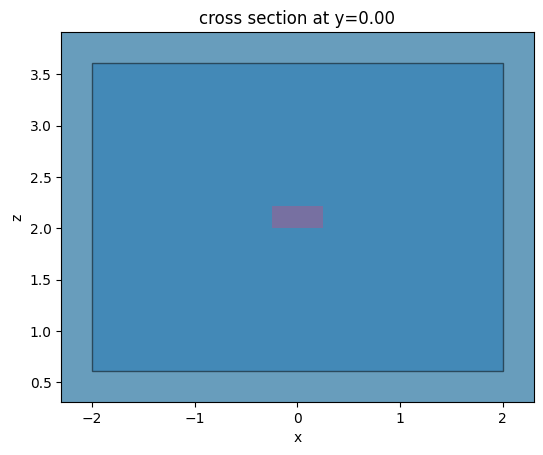
Visual validation of the setup.
[9]:
scene.plot(y=0, hlim=[-w_sim / 2, w_sim / 2], vlim=[z_sim - h_sim / 2, z_sim + h_sim / 2])
plt.show()
Setup Heat Simulation#
We assume that the bottom of the wafer is maintained at temperature \(T=300\) K and ignore heat transfer at the cladding/air boundary. In this simulation setup these boundary conditions can be set using MediumMediumInterface placement. Note since no other boundary conditions are specified, the other sides of the simulation box will be treated as insulating boundary conditions.
Convective cooling/heating at the cladding/air boundary can be easily taken into account using ConvectionBC boundary conditions.
[10]:
bc_bottom = td.HeatBoundarySpec(
    placement=td.MediumMediumInterface(mediums=["Si", "air"]),
    condition=td.TemperatureBC(temperature=300),
)

bc_top = td.HeatBoundarySpec(
    placement=td.MediumMediumInterface(mediums=["SiO2", "air"]),
    condition=td.HeatFluxBC(flux=0),
)
Create a uniform heat source inside the heater structure equivalent to electrical current of \(7.3 \times 10^{-3}\) A.
[11]:
current = 7.4e-3  # A
heat_rate = (current / h_heater / w_heater) ** 2 / TiN_sigma  # convert into power
heater_source = td.HeatSource(rate=heat_rate, structures=[heater.name])
We will measure temperature distribution in the entire cross section of the simulation setup. Note that in this example we request to return heat solver results on the original unstructured grid.
[12]:
temp_mnt = td.TemperatureMonitor(size=(td.inf, 0, td.inf), name="temperature", unstructured=True)
For spatial discretization we will use a distance-based meshing specifying that solid-solid material interfaces should be discretized with mesh size equal to the heater height h_heater divided by 3 and away from interfaces the grid should coarsen to four times of that size. Setting distance_interface to three of minimal mesh size will create approximately three layers of cells with the minimal size around interfaces. Cells outside of this region will have sizes according to linear
relation dl_interface * (1 - ratio(d)) + dl_interface * ratio(d), where ratio(d) = (d - distance_interface) / (distance_bulk - distance_interface) and d is the distance to the closest material interface. We choose this transition to happen on the order of 2 * d_heater. We will also exclude using the higher mesh resolution around the wafer since that region is of less interest.
[13]:
# parameters for meshing
dl_min = h_heater / 3
dl_max = 4 * dl_min

grid_spec = td.DistanceUnstructuredGrid(
    dl_interface=dl_min,
    dl_bulk=dl_max,
    distance_interface=3 * dl_min,
    distance_bulk=2 * d_heater,
    non_refined_structures=["wafer"],  # do not refine near wafer
)
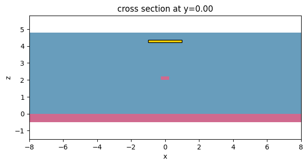
Pack components into a heat simulation specification. Note that from the heat transfer perspective the problem is symmetric around \(x=0\). Thus, we can set symmetry specification to (1, 0, 0) to reduce simulation size and cost.
[14]:
heat_sim_buffer = 2
[15]:
heat_sim = td.HeatChargeSimulation.from_scene(
    scene=scene,
    center=(0, 0, z_sim),
    size=(w_sim + heat_sim_buffer * 2, 0, h_sim),
    boundary_spec=[bc_bottom, bc_top],
    sources=[heater_source],
    monitors=[temp_mnt],
    symmetry=(1, 0, 0),
    grid_spec=grid_spec,
)
[16]:
heat_sim.plot(y=0.0)
plt.show()
Mesh Inspection#
Before proceeding to submitting a parameter sweep batch we run one simulation and inspect its mesh and solution.
[17]:
job = web.Job(simulation=heat_sim, task_name="heat_sim_check_mesh")
heat_sim_data = job.run()
↓ simulation_data.hdf5.gz ━━━━━━━━━━━ 100.0% • 396.5/396.5 • 52.1 MB/s • 0:00:00
                                               kB
12:41:40 UTC Loading results from simulation_data.hdf5
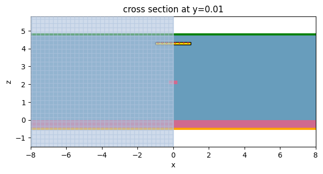
Since while setting up the temperature monitor we requested to return data on unstructured grid, we can plot the associated monitor data to visualize both the solver mesh and the solution. For more information about working with unstructured datasets please refer to the tutorial on unstructured data classes.
[18]:
_, ax = plt.subplots(3, 1, figsize=(10, 10))

heat_sim.plot_structures_heat_conductivity(y=0, alpha=0.5, ax=ax[0])
heat_sim_data["temperature"].temperature.plot(ax=ax[0], field=False)
ax[0].set_xlim([-8, 8])

heat_sim_data["temperature"].temperature.plot(ax=ax[1], grid=False)
ax[1].set_xlim([-8, 8])

heat_sim_data["temperature"].temperature.plot(ax=ax[2])
ax[2].set_xlim([-8, 8])

plt.show()
12:41:41 UTC WARNING: This function 'plot_structures_heat_conductivity' is
             deprecated and will be discontinued. In its place you can use
             plot_structures_heat_charge_property(property="heat_conductivity")
Batch Processing of Heat Simulations#
Having ensured that the simulation mesh is suitable for this simulation setup, let us perform a sweep through several values of electric current in the heating strip. To do this we create a dictionary of simulations with different source definitions.
[19]:
currents = np.linspace(1e-10, 7.4e-3, 10)
heat_sims = {}

for ind, current in enumerate(currents):
    heat_rate = (current / h_heater / w_heater) ** 2 / TiN_sigma
    heater_source = td.HeatSource(rate=heat_rate, structures=[heater.name])

    heat_sim_new = heat_sim.updated_copy(sources=[heater_source])
    heat_sims[f"heat_wg_current_{ind}"] = heat_sim_new
And submit this dictionary using Batch functionality.
[20]:
batch = web.Batch(simulations=heat_sims)
[21]:
batch_data = batch.run()
heat_wg_curren... → success ━━━━━━━━━━━━━━━━━━━━━━━━━ 100% 0:00:06
heat_wg_curren... → success ━━━━━━━━━━━━━━━━━━━━━━━━━ 100% 0:00:06
heat_wg_curren... → success ━━━━━━━━━━━━━━━━━━━━━━━━━ 100% 0:00:06
heat_wg_curren... → success ━━━━━━━━━━━━━━━━━━━━━━━━━ 100% 0:00:06
heat_wg_curren... → success ━━━━━━━━━━━━━━━━━━━━━━━━━ 100% 0:00:06
heat_wg_curren... → success ━━━━━━━━━━━━━━━━━━━━━━━━━ 100% 0:00:06
heat_wg_curren... → success ━━━━━━━━━━━━━━━━━━━━━━━━━ 100% 0:00:06
heat_wg_curren... → success ━━━━━━━━━━━━━━━━━━━━━━━━━ 100% 0:00:06
heat_wg_curren... → success ━━━━━━━━━━━━━━━━━━━━━━━━━ 100% 0:00:06
heat_wg_curren... → success ━━━━━━━━━━━━━━━━━━━━━━━━━ 100% 0:00:06
12:43:29 UTC Batch complete.
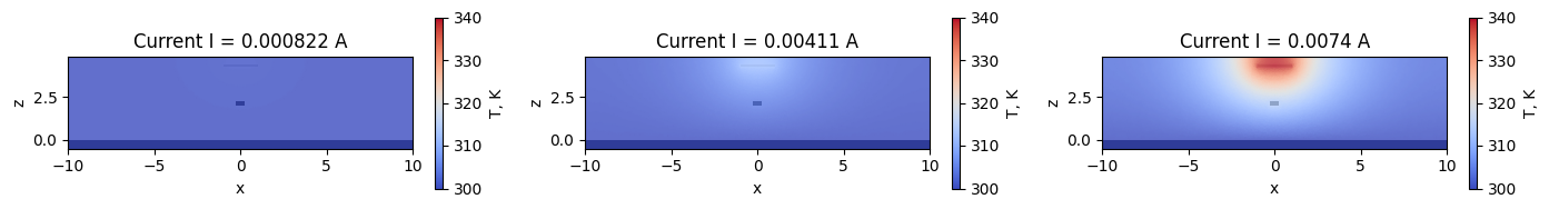
Visualize some of the simulation results.
[22]:
# max temperature value when plotting to enforce the same coloring
temp_max_plot = 340

fig, ax = plt.subplots(1, 3, figsize=(17, 2))

batch_data["heat_wg_current_1"].plot_field("temperature", ax=ax[0], vmax=temp_max_plot)
ax[0].set_title(f"Current I = {currents[1]:1.3} A")

batch_data["heat_wg_current_5"].plot_field("temperature", ax=ax[1], vmax=temp_max_plot)
ax[1].set_title(f"Current I = {currents[5]:1.3} A")

batch_data["heat_wg_current_9"].plot_field("temperature", ax=ax[2], vmax=temp_max_plot)
ax[2].set_title(f"Current I = {currents[9]:1.3} A")

plt.show()
Coupling to Optic Simulations#
Now let us create optic simulations where material properties are modified according to obtained temperature distributions. One can conveniently do that using method .perturbed_mediums_copy() of classes Scene and Simulation. We will use obtained optic simulations only to investigate waveguide
modes, thus we are defining neither sources nor monitors, and only provide grid specification.
[23]:
wvl_um = 1.55
freq0 = td.C_0 / wvl_um

grid_spec = td.GridSpec.auto(min_steps_per_wvl=50, wavelength=wvl_um)

optic_sim = td.Simulation.from_scene(
    scene=scene,
    center=(0, 0, z_sim),
    size=(w_sim, dl_min, h_sim),
    run_time=1e-15,
    grid_spec=grid_spec,
)
Now we can use its grid as the target grid to interpolate the temperature fields to. Note that even though the temperature field is given on an unstructured grid it can be passed to an optic simulation in the same way as Cartesian data arrays.
[24]:
target_grid = optic_sim.grid.boundaries
perturb_sims = []

for _, hs_data in batch_data.items():
    psim = optic_sim.perturbed_mediums_copy(temperature=hs_data["temperature"].temperature)
    perturb_sims.append(psim)
Define plane where waveguide modes will be calculated.
[25]:
mode_plane = td.Box(center=(0, 0, z_core), size=(4, 0, 3))
Visual inspection.
[26]:
fig, ax = plt.subplots(1, 1)
perturb_sims[0].plot(y=0, ax=ax)
mode_plane.plot(y=0, ax=ax, alpha=0.5)
plt.show()
We will use Tidy3D’s mode solver plugin.
[27]:
from tidy3d.plugins.mode import ModeSolver
Find only the first mode at the frequency corresponding to 1.55 um wavelength. Note that simulation objects that are passed to the mode solver contain custom medium data in this case. Sometimes this can lead to large amounts of uploaded/downloaded data. To avoid that, the mode solver web API by default restricts passed simulation object containing custom mediums to mode solver plane only. When that happens, a warning is displayed.
[38]:
mode_solvers = {}

for i, psim in enumerate(perturb_sims):
    ms = ModeSolver(
        simulation=psim,
        plane=mode_plane,
        mode_spec=td.ModeSpec(num_modes=1, precision="double"),
        freqs=[freq0],
    )

    mode_solvers[str(i)] = ms
[29]:
mode_data = web.Batch(simulations=mode_solvers, reduce_simulation=True).run()
0               → success ━━━━━━━━━━━━━━━━━━━━━━━━━ 100% 0:00:07
1               → success ━━━━━━━━━━━━━━━━━━━━━━━━━ 100% 0:00:07
2               → success ━━━━━━━━━━━━━━━━━━━━━━━━━ 100% 0:00:07
3               → success ━━━━━━━━━━━━━━━━━━━━━━━━━ 100% 0:00:07
4               → success ━━━━━━━━━━━━━━━━━━━━━━━━━ 100% 0:00:07
5               → success ━━━━━━━━━━━━━━━━━━━━━━━━━ 100% 0:00:06
6               → success ━━━━━━━━━━━━━━━━━━━━━━━━━ 100% 0:00:06
7               → success ━━━━━━━━━━━━━━━━━━━━━━━━━ 100% 0:00:06
8               → success ━━━━━━━━━━━━━━━━━━━━━━━━━ 100% 0:00:06
9               → success ━━━━━━━━━━━━━━━━━━━━━━━━━ 100% 0:00:06
12:45:52 UTC Batch complete.
Extract found propagation indices into a single array.
[39]:
n_eff = np.array([md.n_eff.isel(f=0, mode_index=0) for md in mode_data.values()])
We will compare to results obtained using different thermal and mode solvers.
[40]:
currents_ref = np.linspace(0.0, 7.4e-3, 10)
neff_ref = [
    2.4401133396065293,
    2.440149458129956,
    2.440257814666438,
    2.4404384121136413,
    2.4406912552977094,
    2.441016350968344,
    2.441413707791896,
    2.4418833363425283,
    2.4424252490914293,
    2.443039460394046,
]
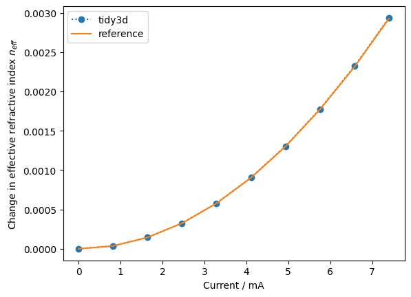
The absolute values of propagation indices are quite sensitive to the type of solver used and parameters of mode solver solution domain. Thus, we compare changes to the propagation indices rather then their absolute values.
[41]:
print(f"Phase shift over 320um: {2 * np.pi / 1.55 * (n_eff[-1] - n_eff[0]) * 320}")
print(f"Phase shift over 320um (ref): {2 * np.pi / 1.55 * (neff_ref[-1] - neff_ref[0]) * 320}")
plt.plot(currents * 1e3, n_eff[:] - n_eff[0], "o:")
plt.plot(currents_ref * 1e3, np.array(neff_ref) - neff_ref[0])
plt.xlabel("Current / mA")
plt.ylabel("Change in effective refractive index $n_{eff}$")
plt.legend(["tidy3d", "reference"])
plt.show()
Phase shift over 320um: 3.747503841548326
Phase shift over 320um (ref): 3.795687048084378
[ ]: