Introduction to heat solver#
This notebook demonstrates basic usage of Tidy3D’s heat solver. We will consider three simple multimaterial setups, planar, cylindrical, and spherical, and compare results to analytical solutions.
Tidy3D’s heat feature solves a steady-state heat equation:
with temperature and flux continuity conditions on the interfaces between different materials:
and subject to a set of boundary conditions on the simulation domain boundary consisting of the following types:
Temperature (Dirichlet): \(\displaystyle T = T_0\)
Heat flux (Neumann): \(\displaystyle k \frac{\partial T}{\partial n} = f\)
Convection (Robin): \(\displaystyle k \frac{\partial T}{\partial n} = c (T-T_0)\)
Here, \(k\) is the thermal conductivity, \(s\) is the volumetric heat source, \(T_0\) is the prescribed temperature value, \(f\) is the prescribed heat flux, and \(c\) is the convection heat transfer coefficient.
Package tidy3d contains all necessary API for defining and running heat simulation on our servers. Note that to use full visualization capabilities of heat solver data one needs package vtk. To install a compatible version of vtk one can use pip install tidy3d[vtk] command.
[1]:
import matplotlib.pyplot as plt
import numpy as np
import tidy3d as td
import tidy3d.web as web
Defining Simulation Scene#
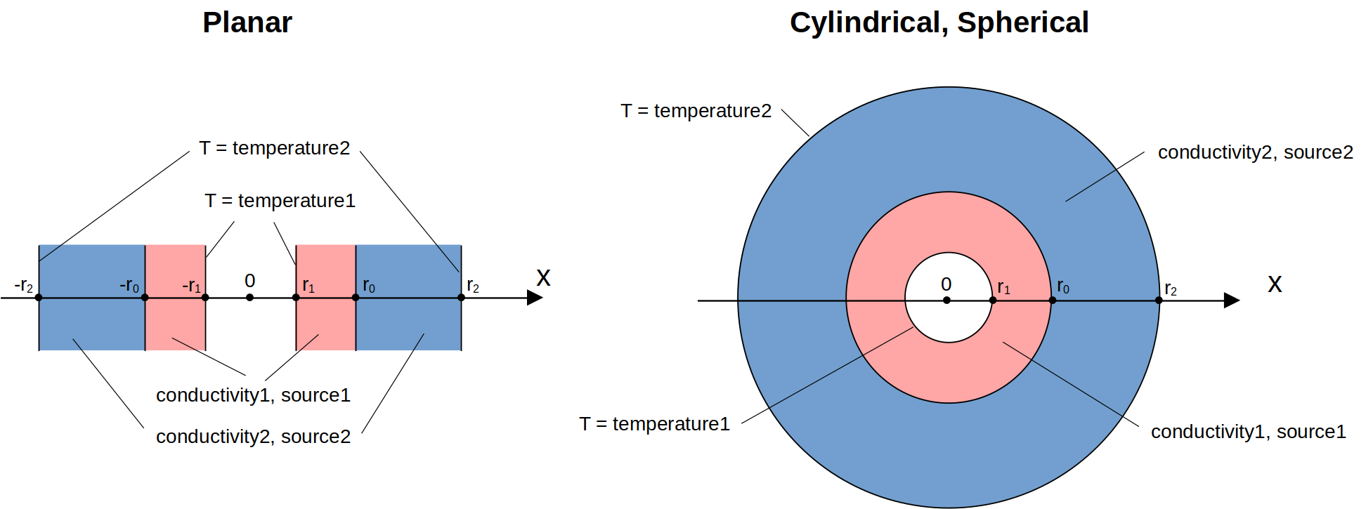
First, we define basic parameter of the simulation setups. In all three cases, we will consider two material layers: one from coordinate r1 to r0, and the second one from r0 to r2. Thermal conductivities of the two layers are defined by parameters conductivity1 and conductivity2. Each layer contains a volumetric heat source with rate given by source1 and source2, correspondingly. Finally, the temperature at the bottom of the first layer is set to temperature1
while the temperature at the top of the second layer is temperature2. Parameters must be provided in units consistent with the spatial units used in Tidy3D, microns. In these tests we do not simulate some specific material, thus, vales of material properties are rather arbitrary.
[2]:
# basic parameters of simulation setups
r1 = 0.2  # um
r0 = 0.5  # um
r2 = 0.9  # um
conductivity1 = 15  # W / (um * K)
conductivity2 = 2  # W / (um * K)
source1 = 1000  # J / (um^3 * K)
source2 = 300  # J / (um^3 * K)
temperature1 = 400  # K
temperature2 = 300  # K
To create materials for heat simulations, one must use heat_spec field of medium classes. Acceptable types for this field are SolidSpec and FluidSpec that define solid and fluid materials from the point of view of heat simulation. Note that the heat equation is only solved inside materials with
SolidSpec, regions with FluidSpec or for which heat_spec is not provided at all are excluded in heat solver. Note that since currently Tidy3D supports only steady-state heat simulation parameter capacity will not have an effect on simulation results.
[3]:
medium1 = td.Medium(
    heat_spec=td.SolidSpec(
        capacity=1,
        conductivity=conductivity1,
    ),
    name="solid1",
)

medium2 = td.Medium(
    heat_spec=td.SolidSpec(
        capacity=1,
        conductivity=conductivity2,
    ),
    name="solid2",
)

background_medium = td.Medium(
    heat_spec=td.FluidSpec(),
    name="fluid",
)
Let us first consider constructing structures for the planar case. We define three overlapping boxes, such that in the region from x=0 to x=1 we have a two layers consisting made of materials medium1 and medium2 on the background of background_medium.
[4]:
planar_top_layer = td.Structure(
    geometry=td.Box(center=(0, 0, 0), size=(2 * r2, td.inf, td.inf)),
    medium=medium2,
    name="top_layer",
)

planar_bottom_layer = td.Structure(
    geometry=td.Box(center=(0, 0, 0), size=(2 * r0, td.inf, td.inf)),
    medium=medium1,
    name="bottom_layer",
)

planar_core = td.Structure(
    geometry=td.Box(center=(0, 0, 0), size=(2 * r1, td.inf, td.inf)),
    medium=background_medium,
    name="core",
)
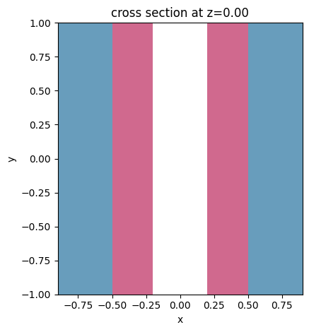
Now we can define a Scene that specifies problem geometry for the planar case and visualize it. The purpose of class Scene is to allow visualization of simulation setups without providing physics-specific details such as sources, monitors, grid specifications, etc, and to provide an easy way to transfer simulation setups between different solvers.
[5]:
scene_planar = td.Scene(
    structures=[planar_top_layer, planar_bottom_layer, planar_core],
    medium=background_medium,
)
Note that by default the region of plotting is determined automatically based on present in Scene structures. If all structures have infinite extent along a given axis (y in this particular case), the plotting limits are set to (-1, 1).
[6]:
scene_planar.plot(z=0)
plt.show()
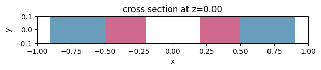
Custom plotting limits can be specified by using arguments vlim and hlim.
[7]:
scene_planar.plot(z=0, vlim=[-0.1, 0.1], hlim=[-1, 1])
plt.show()
Analogously, we create three cylinders and three spheres in cylindrical and spherical cases, respectively. Note, for demonstration purposes we create one of the cylinders as an STL mesh using trimesh package.
[8]:
cyl_top_layer = td.Structure(
    geometry=td.Cylinder(center=(0, 0, 0), length=1, radius=r2),
    medium=medium2,
    name="top_layer",
)

# create a cylinder in STL representation using trimesh
import trimesh

# number of sections along circumference corresponding to resolution 0.2
num_sections = int(np.ceil(2 * np.pi * r0 / 0.02))
cylinder_mesh = trimesh.creation.cylinder(radius=r0, height=1, sections=num_sections)

cyl_bottom_layer = td.Structure(
    geometry=td.TriangleMesh.from_trimesh(cylinder_mesh),
    medium=medium1,
    name="bottom_layer",
)

cyl_core = td.Structure(
    geometry=td.Cylinder(center=(0, 0, 0), length=1, radius=r1),
    medium=background_medium,
    name="core",
)

scene_cyl = td.Scene(
    structures=[cyl_top_layer, cyl_bottom_layer, cyl_core],
    medium=background_medium,
)
[9]:
sphere_top_layer = td.Structure(
    geometry=td.Sphere(center=(0, 0, 0), radius=r2),
    medium=medium2,
    name="top_layer",
)

sphere_bottom_layer = td.Structure(
    geometry=td.Sphere(center=(0, 0, 0), radius=r0),
    medium=medium1,
    name="bottom_layer",
)

sphere_core = td.Structure(
    geometry=td.Sphere(center=(0, 0, 0), radius=r1),
    medium=background_medium,
    name="core",
)

scene_sphere = td.Scene(
    structures=[sphere_top_layer, sphere_bottom_layer, sphere_core],
    medium=background_medium,
)
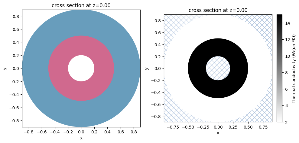
Note that besides function .plot() that paints structures with colors not related to physical properties, there is also function .plot_heat_charge_property(property="heat_conductivity") that uses the heat conductivity of each structure to select a grayscale color for it. Note that regions where the heat equation is not solved (FluidSpec or heat_spec=None) are displayed using light blue
hatching.
[10]:
fig, ax = plt.subplots(1, 2, figsize=(10, 5))
scene_cyl.plot(z=0, ax=ax[0])
scene_sphere.plot_heat_charge_property(property="heat_conductivity", z=0, ax=ax[1])
plt.tight_layout()
plt.show()
Defining Heat Simulation#
Now we proceed to defining a specification for actual heat simulations. We begin with setting simulation domain sizes for each case. Since planar and cylindrical cases are essentially one- and two-dimensional setups, correspondingly, we set a small domain size along invariant directions.
[11]:
# simulation domain parameters

planar_sim_center = (0, 0, 0)
planar_sim_size = (2, 0.1, 0.1)

cyl_sim_center = (0, 0, 0)
cyl_sim_size = (2, 2, 0.1)

sphere_sim_center = (0, 0, 0)
sphere_sim_size = (2, 2, 2)
Boundary Conditions#
Boundary conditions for heat simulation are defined using class HeatBoundarySpec that has two required field condition and placement. The first one defines what boundary conditions should be imposed and accept types TemperatureBC,
HeatFluxBC, or ConvectionBC. While the second one specifies where exactly it should be applied. Available options for that are:
StructureBoundary: boundary of a structure. Only the portion of boundary not covered by subsequent structures is implied.
StructureStructureInterface: interface between two structures. Specifically, the portion of boundary of the succeeding structure inside the preceding structure is implied.
MediumMediumInterface: interface between two media.
SimulationBoundary: boundary of heat simulation domain. Note that specific surfaces of simulation box can be chosen using field
surfaces. For example:SimulationBoundary(surfaces=["z+", "z-"]). By default, all surfaces are selected.StructureSimulationBoundary: part of boundary of heat simulation domain covered by a structure. Again, only the portion of boundary not covered by subsequent structures is implied.
Note that to point at a particular structure or medium, one must set in their definitions field name and use it when creating a boundary condition placement.
For these simulations we set temperature boundary conditions on the top of upper layer and the bottom of the lower layer. We also explicitly set adiabatic boundary conditions on the simulation domain boundary. Note that any solution domain boundaries, which include simulation domain boundary and boundaries facing mediums with empty or FluidSpec type heat_spec, are assigned adiabatic boundary
conditions if no other boundary conditions is specified. Thus, setting adiabatic boundary conditions on the simulation domain boundary is not necessary in these simulations and is only done for demonstration purposes.
[12]:
bc_side = td.HeatBoundarySpec(
    condition=td.HeatFluxBC(flux=0),
    placement=td.SimulationBoundary(),
)

bc_top = td.HeatBoundarySpec(
    condition=td.TemperatureBC(temperature=temperature2),
    placement=td.StructureBoundary(structure="top_layer"),
)

bc_bottom = td.HeatBoundarySpec(
    condition=td.TemperatureBC(temperature=temperature1),
    placement=td.StructureStructureInterface(structures=["core", "bottom_layer"]),
)
Note also that, for example, in case of bc_bottom we could have equivalently set placement to be td.StructureBoundary(structure="core") or td.MediumMediumInterface(mediums=["solid1", "fluid"]).
Sources#
We define volumetric heat source in each of the layers using HeatSource. Similarly to boundary conditions placement, heat sources are assigned to structures by using their names.
[13]:
source_bottom = td.HeatSource(structures=["bottom_layer"], rate=source1)
source_top = td.HeatSource(structures=["top_layer"], rate=source2)
Monitors#
Like in optic Tidy3D simulations, the results of calculations are stored using monitors. Currently, heat simulations support TemperatureMonitor that record spatial temperature distributions in chosen rectangular region. For convenience, even though the heat equation is solved on unstructured grids,
TemperatureMonitor’s can return simulation results on equivalent Cartesian grids in the form of SpatialDataArray. If the results on the original unstructured grid is desired, option unstructured=True can be used. In this case, the data will be presented in the form of
TriangularGridDataset (for planar monitors) or TetrahedralGridDataset (for volumetric monitors). For more information about working with unstructured datasets please refer to the tutorial on unstructured data
classes.
[14]:
temp_mnt = td.TemperatureMonitor(
    center=(0, 0, 0), size=(td.inf, td.inf, 0), name="temperature", unstructured=True
)
HeatChargeSimulation class#
Combining purely geometric information about the simulation setup (Scene) and heat solver specific definitions we can create HeatChargeSimulation instance for each of the three cases. Structures and background medium of a
Scene can either passed directly to a HeatChargeSimulation instance or a convenience method .from_scene() can be used. Note that in these examples we can make use of field symmetry to reduce the size and cost of simulations.
[15]:
heat_sim_planar = td.HeatChargeSimulation(
    center=planar_sim_center,
    size=planar_sim_size,
    medium=scene_planar.medium,
    structures=scene_planar.structures,
    boundary_spec=[bc_top, bc_bottom, bc_side],
    sources=[source_bottom, source_top],
    grid_spec=td.UniformUnstructuredGrid(dl=0.02),
    monitors=[temp_mnt],
    symmetry=(1, 0, 0),
)

heat_sim_cyl = td.HeatChargeSimulation.from_scene(
    center=cyl_sim_center,
    size=cyl_sim_size,
    scene=scene_cyl,
    boundary_spec=[bc_top, bc_bottom, bc_side],
    sources=[source_bottom, source_top],
    grid_spec=td.UniformUnstructuredGrid(dl=0.02),
    monitors=[temp_mnt],
    symmetry=(1, 1, 0),
)

heat_sim_sphere = td.HeatChargeSimulation.from_scene(
    center=sphere_sim_center,
    size=sphere_sim_size,
    scene=scene_sphere,
    boundary_spec=[bc_top, bc_bottom, bc_side],
    sources=[source_bottom, source_top],
    grid_spec=td.UniformUnstructuredGrid(dl=0.02),
    monitors=[temp_mnt],
    symmetry=(1, 1, 1),
)
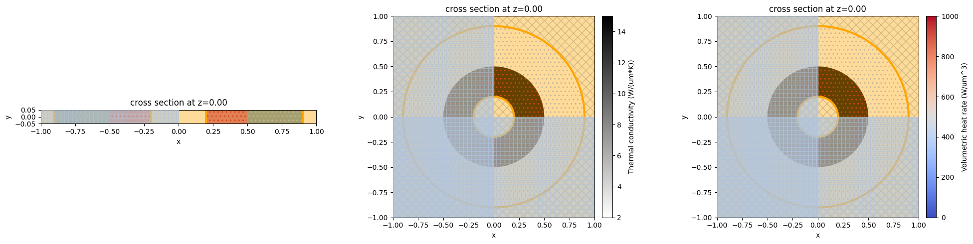
Plotting function of HeatChargeSimulation displays heat conductivity information of structures using gray scale colors, assigned boundary conditions using thick lines (orange for TemperatureBC, green for
HeatFluxBC, and brown for ConvectionBC), and heat sources as colored dots. Specifying colorbar="conductivity" or colorbar="source" changes the colorbar accordingly.
[16]:
fig, ax = plt.subplots(1, 3, figsize=(20, 5))
heat_sim_planar.plot(z=0, ax=ax[0])
heat_sim_cyl.plot_property(property="heat_conductivity", z=0, ax=ax[1])
heat_sim_sphere.plot_property(property="source", z=0, ax=ax[2])
plt.tight_layout()
plt.show()
Solving#
Now we can submit the three heat simulation to our servers for solving. Heat simulations share the same web API as optic simulations. That is, we can submit simulations to servers in three ways.
The first way is to use function web.run(), which returns simulation results as a HeatChargeSimulationData instance.
[17]:
heat_sim_data_planar = web.run(simulation=heat_sim_planar, task_name="heat_sim_planar")
10:11:43 UTC Loading simulation from local cache. View cached task using web UI
             at
             'https://tidy3d.simulation.cloud/workbench?taskId=hec-65777f17-0524
             -4a6f-b309-a3992dc0dc22'.
Alternatively, one can use Job container.
[18]:
job = web.Job(simulation=heat_sim_cyl, task_name="heat_sim_cyl")
Note: This way, we can check the estimated cost before running the simulation.
[19]:
estimate_cost = job.estimate_cost()
             Loading simulation from local cache. View cached task using web UI
             at
             'https://tidy3d.simulation.cloud/workbench?taskId=hec-838feef2-c7ef
             -4204-bccb-14f6fd8a420e'.
Now run the simulation.
[20]:
heat_sim_data_cyl = job.run()
real_cost = job.real_cost()
10:11:44 UTC WARNING: Warning messages were found in the solver log. For more
             information, check 'SimulationData.log' or use
             'web.download_log(task_id)'.
10:11:45 UTC Billed flex credit cost: 0.025.
Finally, class Batch facilitates a convenient submission of multiple simulations. Let us, for example, submit the spherical case at several different mesh resolutions.
[21]:
dl_refine = [0.04, 0.02, 0.01, 0.005]
heat_sim_sphere_refine = {
    "heat_sim_sphere_" + str(dl): heat_sim_sphere.updated_copy(
        grid_spec=td.UniformUnstructuredGrid(dl=dl)
    )
    for dl in dl_refine
}
[22]:
batch = web.Batch(simulations=heat_sim_sphere_refine)
estimate_cost = batch.estimate_cost()
             No Flexcredit cost for batch as all simulations were restored from
             local cache.
[23]:
batch_data = batch.run()
real_cost = batch.real_cost()
Found all simulations in cache.
10:11:48 UTC Total billed flex credit cost: 0.100.
[24]:
heat_sim_data_sphere = batch_data["heat_sim_sphere_0.02"]
For more details on Tidy3D’s web API see the corresponding tutorial.
Data Visualization and Analysis#
The solution data to the heat equation is stored in HeatChargeSimulationData object. Its field .data contains HeatMonitorData instances corresponding to each monitor from HeatChargeSimulation.monitor. Note that the heat equation is solved on an unstructured mesh, however, for a more convenient manipulation of data in the Tidy3D python client, the solution results can be
transferred onto a Cartesian grid. If the results on the original unstructured grid is desired, option unstructured=True in monitor setup can be used. In that case, the data would be presented in the form of TriangularGridDataset (for planar monitors) or
TetrahedralGridDataset (for volumetric monitors). For more information about working with unstructured datasets please refer to the tutorial on unstructured data classes.
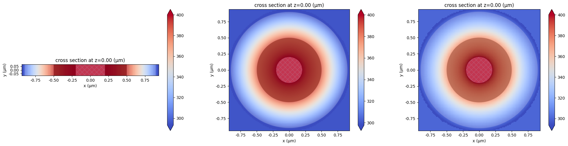
Temperature distribution corresponding to a given monitor can be visualized using function HeatChargeSimulationData.plot_field(). Note that numerical solutions are slightly extrapolated outside of solution domains, such that interpolation can be accurately performed anywhere in the vicinity of the solution domain. Additionally, data in monitor data objects are automatically expanded with the respect to the symmetry of the original simulation.
[25]:
fig, ax = plt.subplots(1, 3, figsize=(20, 5))

heat_sim_data_planar.plot_field("temperature", ax=ax[0])

heat_sim_data_cyl.plot_field("temperature", ax=ax[1])

heat_sim_data_sphere.plot_field("temperature", ax=ax[2])

plt.tight_layout()
plt.show()
Now let us compare the numerical results to analytical solutions. The general solution to the quasi one-dimensional steady-state heat equation in 1, 2 and 3 dimensions can be written as
where \(N\) is the problem’s dimensionality, \(s\) is the source term, \(k\) is the heat conductivity, \(A\) and \(B\) are coefficients defined by boundary conditions, and \(u_N(r)\) is the Green function, which is given by
in one, two, and three dimensions, respectively.
The analytical solutions \(T(r)\) for the considered two-layer setups can be decomposed into two parts \(T_1(r)\) and \(T_2(r)\) such that
and each of which are given by the form \(T_a(r)\) but with different coefficients \(A_1\), \(B_1\) and \(A_2\), \(B_2\). These are defined from boundary conditions:
Thus, coefficients \(A_1\), \(A_2\), \(B_1\), and \(B_2\) can be found by solving linear system
[26]:
# green functions of steady state heat equations in 1, 2, and 3 dimensions
u = [
    lambda r: r,
    lambda r: np.log(r),
    lambda r: -1.0 / r,
]

#  and their derivatives
du = [
    lambda r: 1,
    lambda r: 1.0 / r,
    lambda r: 1.0 / r**2,
]
Let us define a helper function that finds coefficients \(A\) and \(B\) from given boundary conditions.
[27]:
def get_coeffs(u, du, N):
    """A helper function that finds coefficients of analytical solution in N dimensions."""

    # construct matrix
    mat = [
        [u(r1), 1, 0, 0],
        [0, 0, u(r2), 1],
        [u(r0), 1, -u(r0), -1],
        [conductivity1 * du(r0), 0, -conductivity2 * du(r0), 0],
    ]

    # construct right-hand side
    rhs = [
        temperature1 + 0.5 / N * source1 / conductivity1 * r1**2,
        temperature2 + 0.5 / N * source2 / conductivity2 * r2**2,
        0.5 / N * r0**2 * (source1 / conductivity1 - source2 / conductivity2),
        2 * 0.5 / N * r0 * (source1 - source2),
    ]

    A1, B1, B2, A2 = np.linalg.solve(mat, rhs)

    return A1, B1, B2, A2
And another helper function that samples analytical solution at given coordinate points.
[28]:
def get_analytical(N, x):
    """A helper function that samples N-dimensional analytical solution at coordinates x."""

    A1, B1, A2, B2 = get_coeffs(u[N - 1], du[N - 1], N)

    x1_inds = np.logical_and(np.abs(x) >= r1, np.abs(x) < r0)
    x2_inds = np.logical_and(np.abs(x) >= r0, np.abs(x) <= r2)

    x1 = x[x1_inds]
    x2 = x[x2_inds]

    T1 = -0.5 / N * source1 / conductivity1 * x1**2 + A1 * u[N - 1](np.abs(x1)) + B1
    T2 = -0.5 / N * source2 / conductivity2 * x2**2 + A2 * u[N - 1](np.abs(x2)) + B2

    return np.concatenate((x1, x2)), np.concatenate((T1, T2))
Now we can easily find analytical solution for each of the cases and compare them to the numerical ones. Let us first perform this comparison for all three cases at resolution dl = 0.02.
[29]:
# For unstructured data, we first slice to get xarray DataArray, then access coords
line_data_planar = heat_sim_data_planar["temperature"].temperature.sel(y=0).squeeze()
x = line_data_planar.coords["x"].values
x_exact_planar, temperature_exact_planar = get_analytical(1, x)

line_data_cyl = heat_sim_data_cyl["temperature"].temperature.sel(y=0).squeeze()
x = line_data_cyl.coords["x"].values
x_exact_cyl, temperature_exact_cyl = get_analytical(2, x)

line_data_sphere = heat_sim_data_sphere["temperature"].temperature.sel(y=0).squeeze()
x = line_data_sphere.coords["x"].values
x_exact_sphere, temperature_exact_sphere = get_analytical(3, x)
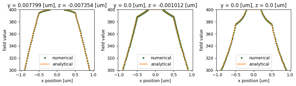
As one can see the solver accurately reproduces analytical solutions.
[30]:
fig, ax = plt.subplots(1, 3, figsize=(10, 3))

ax[0].plot(x_exact_planar, temperature_exact_planar, ".")
heat_sim_data_planar["temperature"].temperature.sel(y=0).plot(ax=ax[0])
ax[0].legend(["numerical", "analytical"])
ax[0].set_ylim([300, 400])

ax[1].plot(x_exact_cyl, temperature_exact_cyl, ".")
heat_sim_data_cyl["temperature"].temperature.sel(y=0).plot(ax=ax[1])
ax[1].legend(["numerical", "analytical"])
ax[1].set_ylim([300, 400])

ax[2].plot(x_exact_sphere, temperature_exact_sphere, ".")
heat_sim_data_sphere["temperature"].temperature.sel(y=0).plot(ax=ax[2])
ax[2].legend(["numerical", "analytical"])
ax[2].set_ylim([300, 400])

plt.tight_layout()
plt.show()
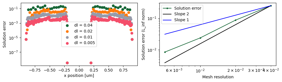
Now, let us look at the convergence of numerical solutions in the spherical case. Plotting the dependence of the solution error (in the \(L_\infty\) norm) on the grid resolution we confirm the second order of convergence of the solver.
[31]:
fig, ax = plt.subplots(1, 2, figsize=(10, 3))
errors = []
for ind, (_, sim_data) in enumerate(batch_data.items()):
    # For unstructured data, slice first then get coords
    line_data = sim_data["temperature"].temperature.sel(z=0, y=0, method="nearest").squeeze()
    line_data = line_data.groupby("x").mean().sortby("x")
    x = line_data.coords["x"].values
    x_exact_sphere, temperature_exact_sphere = get_analytical(3, x)
    # Use xarray interp to get numerical values at exact solution points
    temperature_numerical = line_data.interp(x=x_exact_sphere).values
    error = np.abs(temperature_numerical - temperature_exact_sphere)
    errors.append(np.max(error))
    ax[0].scatter(x_exact_sphere, error, label=f"dl = {dl_refine[ind]}")

ax[0].set_yscale("log")
ax[0].set_xlabel("x position [um]")
ax[0].set_ylabel("Solution error")
ax[0].legend()

ax[1].loglog(dl_refine, errors, ".-", label="Solution error")
ax[1].loglog(
    dl_refine,
    errors[0].data * (np.array(dl_refine) / dl_refine[0]) ** 2,
    "-k",
    label="Slope 2",
)
ax[1].loglog(
    dl_refine,
    errors[0].data * (np.array(dl_refine) / dl_refine[0]),
    "-b",
    label="Slope 1",
)
ax[1].set_xlabel("Mesh resolution")
ax[1].set_ylabel("Solution error (L_inf norm)")
ax[1].legend()

plt.tight_layout()
plt.show()
10:11:51 UTC WARNING: Warning messages were found in the solver log. For more
             information, check 'SimulationData.log' or use
             'web.download_log(task_id)'.
10:11:52 UTC WARNING: Warning messages were found in the solver log. For more
             information, check 'SimulationData.log' or use
             'web.download_log(task_id)'.