Wave Ports

This page discusses how to set up wave ports in Flexcompute RF (also Flex RF).

The wave port is designed to excite one or more propagating modes in the connected port structures. It can also function as a matched absorber for outgoing modes.

There are two types of wave ports: the modal type WavePort and the terminal type TerminalWavePort. They differ mainly in how the propagating modes are selected, and how the port reference impedance is defined.

Wave port or lumped port?

Wave ports excite the actual transmission line mode supported by the port cross-section, so they are accurate over the band where that mode is well-defined.

The lumped representation is fundamentally an approximation of physical reality. It is typically most accurate when the port/element size is much smaller than the wavelength ($L \ll \lambda/10$).

Use lumped ports in the following scenarios:

• The port size is much smaller than the wavelength.
• The port structures are not typical transmission lines.
• A quicker but more approximate simulation is desired.

Use wave ports in the following scenarios:

• The port structures are good transmission lines.
• Perfect impedance match for the outgoing wave is desired.
• Calculating the transmission line mode properties in the 2D port plane.

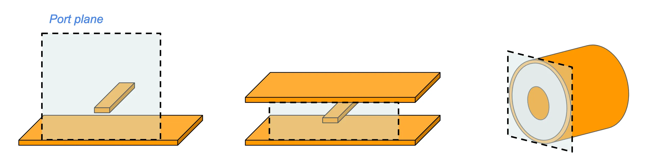
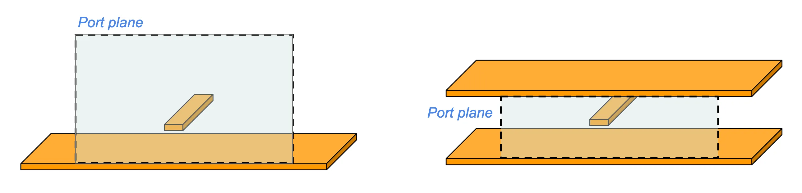
Note: mixing-and-matching lumped and wave ports is generally discouraged unless the different reference impedances and de-embedding standards are carefully handled.

Basic Usage

A wave port is a planar object: its size must have exactly one zero dimension, and the direction field ('+' or '-') sets the direction of mode propagation. The port must always be axis-aligned.

Modal Wave Port

The WavePort excites the propagating modes found by a 2D mode solver in the port plane. Each port-mode combination contributes one row/column of the S-matrix. The characteristic impedance of each mode is used as the reference impedance by default.

For single-mode TEM transmission lines, it is fine to leave most settings at default.

# Minimal wave port definition
my_wave_port = WavePort(
    name='port 1',
    center=(0, 0, -200),
    size=(0, 500, 300),   # Normal is along x-axis
    direction='+',        # Wave travelling in +x direction
)

For multi-ended transmission lines, as well as TE/TM waveguides, more setup is usually necessary. The MicrowaveModeSpec object provides additional settings to the wave port.

# Set number of modes and target index
mode_spec = MicrowaveModeSpec(
    num_modes=2,
    target_neff=2.5,
)
# Assign to wave port
my_wave_port = WavePort(
    ...
    mode_spec=mode_spec,
)

See the API reference page for MicrowaveModeSpec for a full list of options. Some advanced functions are discussed below.

Terminal Wave Port

The TerminalWavePort is suitable for transmission lines with one or more signal traces (e.g. microstrip traces, differential pairs, multi-strip lines). Instead of working in the modal basis, it works in the terminal basis: each conductor in the port plane corresponds to one “terminal”. Voltages and currents are defined per terminal, and the characteristic impedance becomes a terminal-by-terminal matrix that may have off-diagonal coupling.

The minimal setup for the TerminalWavePort is very similar to that for the WavePort.

# Minimal terminal wave port
my_TWP = TerminalWavePort(
    name='port 1',
    center=(0, 0, -200),
    size=(300, 200, 0),
    direction='+',
)

Once defined, conductors fully enclosed by the port plane are auto-detected and labeled as terminals T0, T1, … in left-to-right, bottom-to-top order. Use the plot_port() feature of TerminalComponentModeler to visually inspect the labeling.

# Set up TCM
my_tcm = TerminalComponentModeler(
    ...,
    ports = [my_TWP, ...]
)

# Use plot_port to inspect terminals and diff pairs
my_tcm.plot_port(my_TWP.name)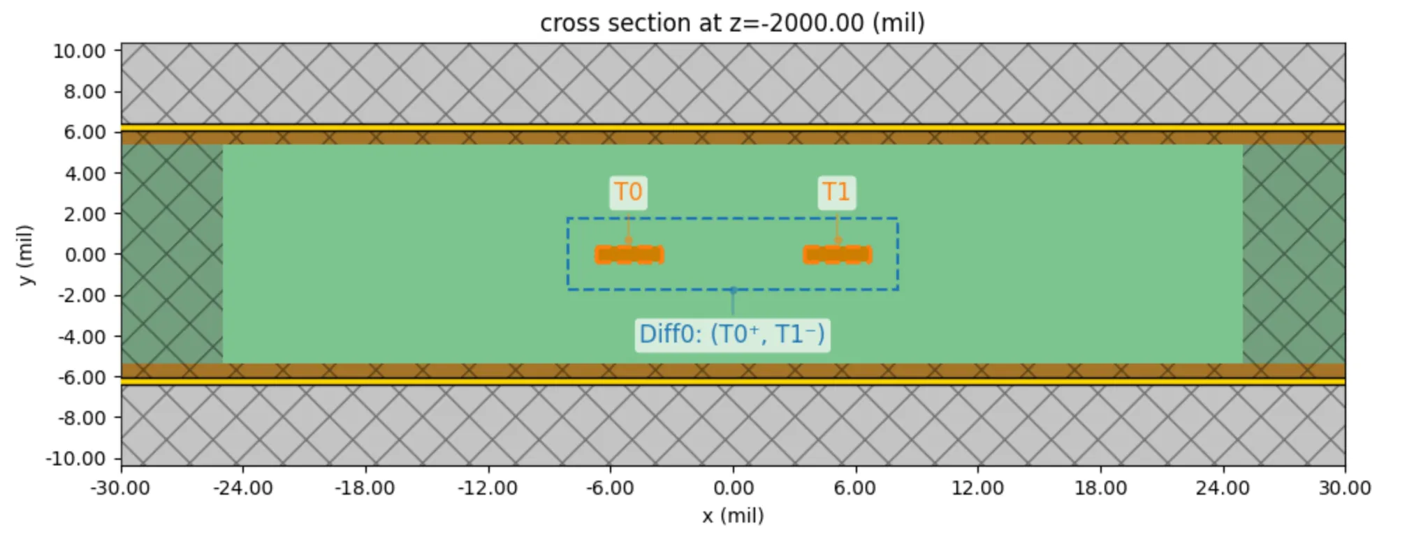

To pair terminals together in a differential/common double-ended configuration, use the differential_pairs parameter.

# Set two terminals as a differential pair
my_TWP = TerminalWavePort(
    ...,
    differential_pairs=[('T0', 'T1')],
)

After grouping, the two single-ended terminals T0 and T1 are replaced by Diff0@comm (common mode) and Diff0@diff (differential mode), each with its own row/column in the S-matrix. Any remaining single-ended terminals (e.g. T2) keep their original labels. See Working with Results for the port/mode indexing scheme.

Previewing the Port with a 2D Mode Solver

Before running a full 3D simulation, it is good practice to verify that the wave port resolves the expected mode(s). Both WavePort and TerminalWavePort expose a to_mode_solver() method that returns a pre-configured ModeSolver. It is only necessary to provide the base Simulation and the desired frequency points.

# Run a 2D mode solver for the wave port and inspect the modes
# Needs: a base Simulation; frequency points for mode solve
mode_solver = my_wave_port.to_mode_solver(
    simulation=sim,
    freqs=np.linspace(f_min, f_max, 41),
)
mode_data = web.run(mode_solver, task_name='wave port mode preview')

# Plot |E| for mode 0 at 1 GHz
mode_solver.plot_field('E', val='abs', mode_index=0, f=1e9)

See Working with Results for more information on analyzing 2D mode data.

Port Setup Guide

When setting up wave port, it is important to consider a few general principles.

First, the port boundaries must be treated as PEC for the purposes of the 2D mode calculation. Any structures which touch/intersect the port boundaries will be considered electrically connected (shorted). This will influence the transmission line modes that can be found using the wave port.

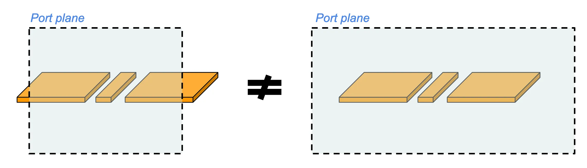
In the figure above, the left and right scenarios are not equivalent. On the left, the port boundaries intersect the side ground planes of the co-planar waveguide (CPW). Thus, the side planes are grounded to the same potential. This is the appropriate setup for finding the typical CPW mode. On the right, the port boundaries do not touch any of the CPW structures. This implies that all three metal structures are at (possibly different) floating potentials, and the found modes would correspond to the parallel wire modes.

Caution

The actual boundary of the wave port can sometimes be one or two grid cells larger than the specified size parameter, which can affect 2D electrical connectivity. It is recommended to:

• Use the TerminalComponentModeler.plot_port() feature to visually inspect each port.
• Run 2D mode solver on each wave port using WavePort.to_mode_solver() or TerminalWavePort.to_mode_solver() to confirm that the desired mode(s) are found.

The second consideration is whether the transmission line is open boundary (e.g. microstrip, CPW) or closed boundary (coaxial).

For open boundary modes, the wave port should be as large as possible to accurately solve for the mode profile. A common rule-of-thumb is that the minimum port size should be 3 to 5 times the signal line dimensions (width and height). When in doubt, check the mode profile using the 2D mode solver to ensure that the mode amplitude falls off sufficiently toward the port boundaries. The same guideline holds for semi-open boundary modes (e.g. stripline).

For closed boundary modes, the port only needs to be large enough to encompass the outer metal enclosure, e.g. the outer conductor of a coaxial line.

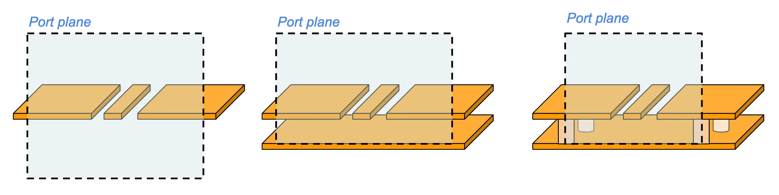
Below, we show some suggested port layouts for common planar transmission lines. The first figure shows the microstrip and stripline.

The next figure shows the port layout for three different types of CPW configurations: open CPW, grounded CPW, and grounded CPW with side vias.

Advanced Usage

Anatomy of a Wave Port

The wave port is not actually a singular, atomic object, but rather a composite object made of several subcomponents.

• Mode source: a mode source that injects the propagating mode at the plane of the active port. There is only one active port in every instance of a port/mode sweep.

• Mode monitor: a monitor at the port plane records the modal amplitudes used to build the S-matrix and other port metrics. This is present on both the active and passive ports.

• PEC frame: a thin PECFrame is placed just behind the source plane to improve mode injection. This is recommended for open-boundary modes (e.g. CPW, microstrip) and can be turned off for closed-boundary modes (e.g. coaxial).

• Mode absorber: a PEC-backed internal absorber added behind the source/monitor plane so that incident waves at the port plane are absorbed. Note that this only applies to specific mode(s) calculated by the absorber. Any non-matching modes will reflected by the PEC backing. The absorber is included by default and can be turned off if the transmission line terminates into PML.

Port Structure Extrusion

When extrude_structures=True, structures that intersect the port plane are extended a few grid cells through the wave port. This should be turned on when the wave port is placed at a location where the surrounding structures are non-invariant in the port normal direction (e.g. at the edge of a board, or bisecting a via).

Mode Sort/Filter

When the mode solver returns multiple modes, the order is set by the sort_spec field of MicrowaveModeSpec. By default, modes are sorted by descending effective index. To filter or sort by a different quantity, pass a ModeSortSpec:

# Keep only modes with TE fraction > 0.5
# then sort by absolute difference from n_eff=1.6 (closer first)
mode_spec = MicrowaveModeSpec(
    num_modes=10,
    sort_spec=ModeSortSpec(
        sort_key = 'n_eff',
        sort_reference = 1.6,
        filter_key='TE_fraction',
        filter_reference=0.5,
        filter_order='over',
        keep_modes='filtered',  # drop modes that fail the filter
    ),
)

Available sort/filter keys: n_eff, k_eff, TE_fraction, TM_fraction, wg_TE_fraction, wg_TM_fraction, mode_area, fill_fraction_box.

Set keep_modes='all' (default) to keep all solved modes with the filtered group placed first, keep_modes='filtered' to drop modes that fail the filter, or an integer to keep that many modes.

Path Integrals

By default, WavePort uses AutoImpedanceSpec to choose voltage and current integration paths automatically based on the detected conductors in the port plane. These path integrals are used to determine the port voltage and current, and by extension, the port reference impedance and S-parameters.

This auto-detection works well for TEM modes with well-defined signal trace profiles. For non-standard transmission lines or TE/TM-based waveguides, you should set up a CustomImpedanceSpec.

# Define a voltage path integral horizontally
# across a rectangular waveguide cross-section
#   --------------------
#  |                    |
#  |--------->>---------|   Voltage integration line
#  |                    |
#   --------------------
voltage_spec = AxisAlignedVoltageIntegralSpec(
    center=(0, 0, 0),
    size=(200, 0, 0),   # integrate along x from -100 to 100
    sign='+',           # left-to-right
)

# Include the voltage spec in the wave port
mode_spec = MicrowaveModeSpec(
    ...,
    impedance_specs=CustomImpedanceSpec(
        voltage_spec=voltage_spec,
    ),
)
my_wave_port = WavePort(
   ...,
   mode_spec=mode_spec
)

For a given impedance spec, you may define a voltage_spec only, a current_spec only, or both. When only one is given, the other is inferred from the modal power flow. Note that the calculated port impedance may differ slightly, corresponding to the V-I, P-I, and P-V conventions.

When more than one mode is included (num_modes > 1), you may pass one single CustomImpedanceSpec to apply for all modes, or a list of one CustomImpedanceSpec per mode.

All path-integral paths must lie strictly inside the port plane.

Mode Interpolation

For broadband simulations where modes vary smoothly with frequency, you can solve the mode equation on a small set of source frequencies and interpolate the result onto the full requested frequency grid using a ModeInterpSpec.

# Solve at 10 uniformly spaced frequencies, interpolate cubically
interp_spec = ModeInterpSpec.uniform(num_points=10, method='cubic')

# Chebyshev nodes + polynomial interpolation (optimal for smooth dispersion)
interp_spec = ModeInterpSpec.cheb(num_points=10)

# Custom sampling frequencies
interp_spec = ModeInterpSpec.custom(
    freqs=[1e9, 5e9, 10e9, 15e9, 20e9],
    method='linear',
)

# Include in the MicrowaveModeSpec
mode_spec = MicrowaveModeSpec(
    ...,
    interp_spec=interp_spec,
)

Set reduce_data=True on the ModeInterpSpec to additionally reduce the stored field data to only the source frequencies - useful when the port field profiles are needed only sparsely in frequency.

Caution

Mode interpolation requires frequency tracking ModeSortSpec.track_freq set, which is the case by default with track_freq='central'. Without tracking, mode ordering can jump between source frequencies and the interpolated result is meaningless.