Intro to Antenna Modeling

Download as:

Quarto (.qmd)

In this notebook, we will demonstrate how to simulate a simple RF antenna and compute key antenna metrics, such as:

• S-parameters
• Impedance
• Field profile
• Directivity and Gain
• Axial Ratio

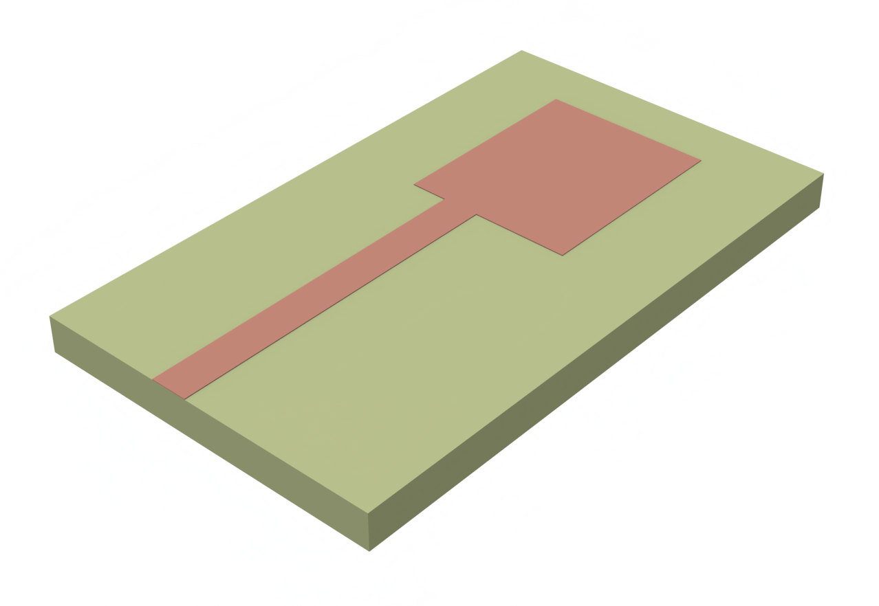
We will use the patch antenna model designed by Sheen et al. in Reference [1]. A rectangular patch antenna is a type of microstrip antenna consisting of a rectangular conductive patch placed on a dielectric substrate with a ground plane on the opposite side. These antennas are widely used in wireless communication applications due to their simple design, ease of fabrication, and low profile.

In [1]:

import flex_rf.tidy3d as rf
import flex_rf.web as web
import matplotlib.colors as colors
import matplotlib.pyplot as plt
import numpy as np
import plotly.graph_objects as go
import plotly.io as pio
rf.config.logging.level = 'ERROR'

# Set plotly default renderers
pio.renderers.default = "plotly_mimetype+notebook_connected"

Building the Model

Units and Frequency Settings

The antenna has a primary resonance at f ~ 7.5 GHz and a secondary resonance near f ~ 10 GHz. We will choose a frequency range that encompasses both resonances.

In [2]:

# Frequency and wavelength parameters
freq_start = 5e9
freq_stop = 11e9
freq0 = (freq_start + freq_stop) / 2
wavelength0 = rf.C_0 / freq0

# Target frequencies (also used to define field monitors)
freqs_target = [7.5e9, 10e9]

# Frequency sweep points (also append target frequencies)
freqs =  np.unique(np.append(np.linspace(freq_start, freq_stop, 201), freqs_target))

In Flex RF, the default units are micrometers (µm) and Hertz (Hz). To work in different length units, we introduce a scaling factor.

In [3]:

# Scaling used for millimeters
mm = 1e3

Materials

The dielectric substrate has a constant relative permittivity of 2.2. The metal structures are represented by the perfect electric conductor (PEC) medium.

In [4]:

# Materials present
medium_air = rf.Medium(permittivity=1.0, name="Air")
medium_sub = rf.Medium(permittivity=2.2, name="Substrate")
medium_metal = rf.PECMedium()

Geometry and Structures

We follow the dimensions outlined in Reference [1] to create the patch antenna.

In [5]:

# Metal thickness
th = 0.05 * mm

# Substrate parameters
sub_x = 23.34 * mm
sub_y = 40 * mm
sub_z = 0.794 * mm

# Patch parameters
patch_x = 12.45 * mm
patch_y = 16 * mm

# Feed line parameters
feed_x = 2.46 * mm
feed_y = 20 * mm
feed_offset = 2.09 * mm

The structures are created below.

In [6]:

# Create substrate
substrate = rf.Structure(
    geometry=rf.Box(center=[0, 0, 0], size=[sub_x, sub_y, sub_z]),
    medium=medium_sub,
    name="Substrate",
)

# Create ground plane
ground_plane = rf.Structure(
    geometry=rf.Box(center=[0, 0, -(sub_z + th) / 2], size=[sub_x, sub_y, th]),
    medium=medium_metal,
    name="Ground",
)

# Create feed line
feed_line = rf.Structure(
    geometry=rf.Box.from_bounds(
        rmin=[-patch_x / 2 + feed_offset, -sub_y / 2, sub_z / 2],
        rmax=[-patch_x / 2 + feed_offset + feed_x, -sub_y / 2 + feed_y, sub_z / 2 + th],
    ),
    medium=medium_metal,
    name="Feed line",
)

# Create patch antenna
patch = rf.Structure(
    geometry=rf.Box.from_bounds(
        rmin=[-patch_x / 2, -sub_y / 2 + feed_y, sub_z / 2],
        rmax=[patch_x / 2, -sub_y / 2 + feed_y + patch_y, sub_z / 2 + th],
    ),
    medium=medium_metal,
    name="Patch",
)

The structures are consolidated into a list below. In Flex RF, overlapping structures are resolved according to their medium type by default: PEC overrides lossy metal overrides dielectrics. Within each medium type, later structures in the list override earlier ones.

In [7]:

# List of structures for the simulations
structures_list = [substrate, ground_plane, feed_line, patch]

Monitors

We define a FieldMonitor to observe the field distribution in the patch antenna plane.

In [8]:

# Field monitor to view the electromagnetic fields in the patch plane
monitor_field = rf.FieldMonitor(
    center=(0, 0, sub_z / 2),
    size=(rf.inf, rf.inf, 0),
    freqs=freqs_target,
    name="field",
)

To obtain radiation characteristics such as directivity and gain, use a DirectivityMonitor. The DirectivityMonitor is set up to surround the entire radiating structure and automatically calculates far-field information through a near-to-far field transformation.

In [9]:

# Define elevation and azimuthal angular observation points
# Theta is the elevation angle and defined relative to global +z axis
theta = np.linspace(0, np.pi, 101)
# Phi is the azimuthal angle and defined relative to global +x axis
phi = np.linspace(0, 2*np.pi, 201)

# Create the DirectivityMonitor
monitor_directivity = rf.DirectivityMonitor(
    size=(30 * mm, 45 * mm, 4 * mm),
    freqs=freqs,
    name="radiation",
    phi=phi,
    theta=theta,
)

Boundaries

The simulation is truncated by Perfectly Matched Layers (PMLs) on all sides by default. PMLs absorb any outgoing radiation. Additionally, we introduce air padding of quarter wavelength thickness around the antenna so that the PMLs do not distort the near field.

In [10]:

# Padding distance
padding = rf.C_0 / freq_start / 4

# Adding padding on each side
sim_x = sub_x + 2 * padding
sim_y = sub_y + 2 * padding
sim_z = sub_z + 2 * padding

Grid/Mesh

The grid specification controls how the simulation domain is discretized. We make use of LayerRefinementSpec to automatically refine the grid near the metal layers. Otherwise, the grid size in the rest of the domain is set automatically according to the wavelength.

In [11]:

# Define layer refinement around antenna plane
lr_spec_1 = rf.LayerRefinementSpec.from_structures(
    structures=[feed_line, patch],         # Refine around these structures
    axis=2,                                # Layer normal is oriented along the z-axis
    min_steps_along_axis = 1,              # 1 grid step along normal direction (thickness)
    corner_refinement=rf.GridRefinement(   # Refined cell size and number around in-plane metal corners
        dl=0.2 * mm, num_cells=2
    ),
)

In [12]:

# Define overall grid specification
grid_spec = rf.GridSpec.auto(
    wavelength=wavelength0, min_steps_per_wvl=20, layer_refinement_specs=[lr_spec_1]
)

Lumped Port

The antenna will be excited by a LumpedPort positioned at the end of the feed line.

In [13]:

# Create a lumped port excitation
port = rf.LumpedPort(
    name="lumped_port",
    center=[-patch_x / 2 + feed_offset + feed_x / 2, -sub_y / 2, 0],
    size=[feed_x, 0, sub_z],
    voltage_axis=2,  # port is aligned with z-axis
    impedance=50,  # port impedance is 50 Ohms
)

Define Simulation and TerminalComponentModeler

The base Simulation object contains all necessary information about the simulation domain that we have defined thus far. Note that the lumped port and the radiation monitor are added later.

The simulation run_time is automatically determined by RunTimeSpec based on the structure quality_factor. For most structures, a value in the range of 3-10 is sufficient. Increase the value for strongly resonant structures, or if high-frequency ripples are present in the S-parameter data.

In [14]:

# Create the simulation object
sim = rf.Simulation(
    size=[sim_x, sim_y, sim_z],
    structures=structures_list,
    monitors=[monitor_field],  # Only near-field monitors; directivity monitor will be added later
    sources=[],  # Sources not needed; lumped port will be added later
    grid_spec=grid_spec,
    run_time=rf.RunTimeSpec(quality_factor=5),  # Automatic run time
    plot_length_units="mm",  # This option will make plots default to units of millimeters.
)

The TerminalComponentModeler automatically conducts a port sweep of the base Simulation in order to generate the full S-parameter matrix as a function of frequency. We specify the port and radiation monitor information here.

In [15]:

# Define TerminalComponentModeler
tcm = rf.TerminalComponentModeler(
    simulation=sim,  # Base simulation to run
    freqs=freqs,  # Sweep frequencies points
    ports=[port],  # Include ports here
    radiation_monitors=[monitor_directivity],  # Include radiation monitors here
)

Examine Structures and Mesh

Before running the simulation, it is advisable to inspect the created structure and mesh.

Here, we examine the simulation domain in the antenna plane, and in the cross-section plane at the terminated end of the feed line (port shown with arrow).

In [16]:

# Create plot
fig, (ax1, ax2) = plt.subplots(1, 2, figsize=(12, 6))

# Plot the structure and mesh in the x-y plane
tcm.plot_sim(
    z=sub_z / 2,
    ax=ax1,
    monitor_alpha=0.2,
)
sim.plot_grid(z=sub_z / 2, ax=ax1, hlim=[-20 * mm, 20 * mm], vlim=[-25 * mm, 25 * mm])

# Plot the structure and mesh in the x-z plane
tcm.plot_sim(
    y=-sub_y / 2,
    ax=ax2,
    monitor_alpha=0.2,
)
sim.plot_grid(y=-sub_y / 2, ax=ax2, hlim=[-15 * mm, 15 * mm], vlim=[-1 * mm, 5 * mm])
ax2.set_aspect(5)

plt.show()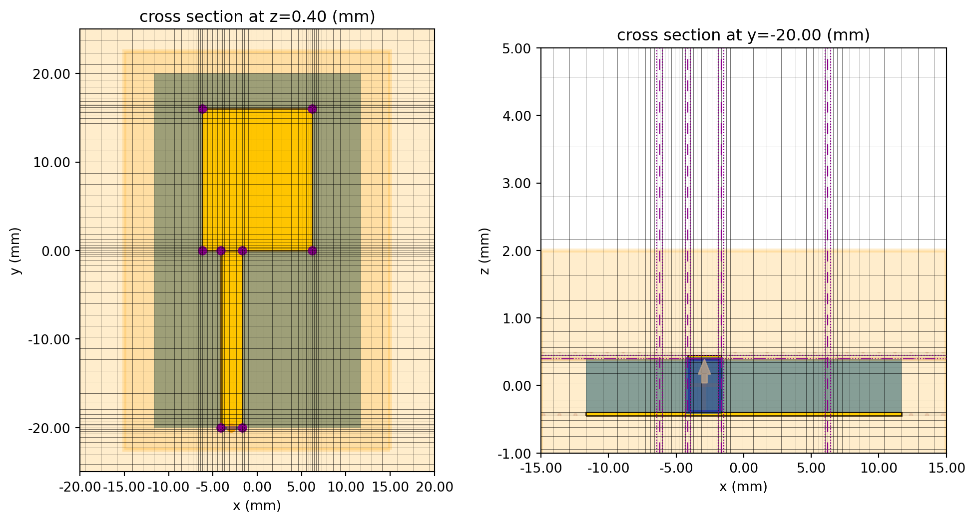

Run simulation

Use the web.run() method to submit the simulation job to the cloud and await results. Switch the verbose flag to True for live job updates.

In [17]:

tcm_data = web.run(tcm, task_name='Antenna tutorial', path='./data/antenna_tutorial.hdf5', verbose=False)

Results

S-parameters

The S-matrix returned by the TerminalComponentModeler is in the shape of fxNxN, where f is the number of frequency points and N is the number of ports. In this case, there is only one port.

Note that Tidy3D uses the physics phase convention. We apply complex conjugate to the calculated S-parameter in order to convert it to the engineering convention.

In [18]:

# Extract the S-matrix from the result data
s_matrix = tcm_data.smatrix()

In [19]:

# Specify port_in and port_out to get the specific S_ij
S11 = np.conjugate(s_matrix.data.isel(port_out=0, port_in=0))

# Transform to dB
S11dB = 20 * np.log10(np.abs(S11))

In [20]:

# Plot S11dB
fig, ax = plt.subplots()
ax.plot(S11dB.f / 1e9, S11dB, "-b",)
ax.set_xlabel("Frequency (GHz)")
ax.set_ylabel("$|S_{11}|$ (dB)")
ax.grid(True)
plt.show()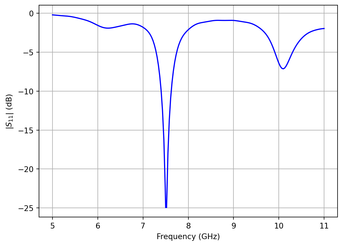

The first and second resonances are clearly visible in the S11 spectrum. Let’s examine the field profile next.

Field Distributions

User-defined monitors record data for every port in the TerminalComponentModeler port sweep. Use a specific port name to access the monitor data corresponding to the port excitation.

In [21]:

# Get simulation data associated with the lumped port excitation
sim_data = tcm_data.data["lumped_port"]

Below, we plot the fields at the first two resonances.

In [22]:

# Plot field monitor data
f, (ax1, ax2) = plt.subplots(1, 2, figsize=(11, 4))
sim_data.plot_field(
    field_monitor_name="field", field_name="Ez", val="abs", f=freqs_target[0], ax=ax1
)
ax1.set_xlim([-10 * mm, 10 * mm])
ax1.set_ylim([-20 * mm, 20 * mm])
ax1.set_title("Electric field distribution at 7.5 GHz")

sim_data.plot_field(
    field_monitor_name="field", field_name="Ez", val="abs", f=freqs_target[1], ax=ax2
)
ax2.set_xlim([-10 * mm, 10 * mm])
ax2.set_ylim([-20 * mm, 20 * mm])
ax2.set_title("Electric field distribution at 10 GHz")
plt.show()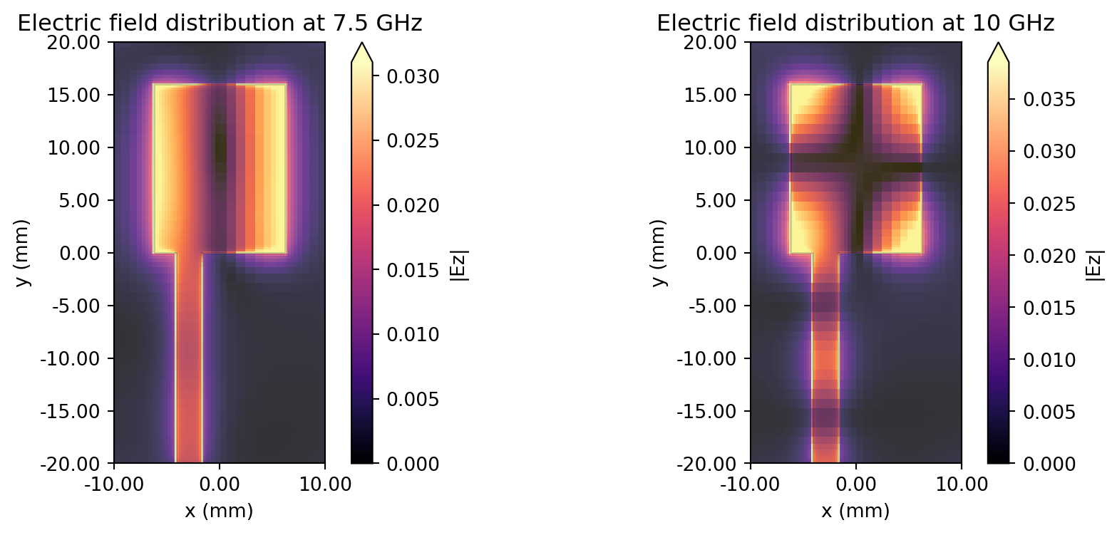

Impedance

The antenna impedance can be calculated from S11.

First, we need to de-embed S11 to account for the length of the feed line. The de-embedding calculation shifts the S11 reference plane from the location of the lumped port ($y = -20$ mm) to the end of the feed line where it connects to the patch ($y = 0$ mm).

In general terms, the de-embedded S-parameter

$$S_\text{de-embedded} = S\exp(2jkL)$$

where $S$ is the original S-parameter, $k$ is the waveguide wavenumber, and $L$ is the shift distance. For simplicity, we assume that the microstrip feed line has a constant effective permittivity of $1.9$ and characteristic impedance of $Z_0=50$ Ohms.

In [23]:

# Wavenumber associated with microstrip feed line
k_microstrip = 2 * np.pi * freqs * np.sqrt(1.9) / rf.C_0

# De-embedded S-parameter
S11_deembedded = S11 * np.exp(1j * 2 * k_microstrip * feed_y)

The antenna impedance can then be calculated using the de-embedded S11.

$$Z_\text{ant} = Z_0 \frac{1+S11_\text{de-embedded}}{1-S11_\text{de-embedded}}$$

In [24]:

# Antenna impedance
Z_ant = 50 * (1 + S11_deembedded) / (1 - S11_deembedded)

Let’s plot the antenna impedance near the first resonance. We observe a very good match with $Z_0$ at resonance.

In [25]:

# Plot antenna impedance near first resonance f=7.5 Ghz
fig, ax = plt.subplots()
ax.plot(freqs / 1e9, np.real(Z_ant), label="Re Z")
ax.plot(freqs / 1e9, np.imag(Z_ant), label="Im Z")
ax.axline((7.5, -50), (7.5, 50), ls="--", color="#555555", label="f=7.5 GHz")
ax.set_xlim(7, 8)
ax.set_ylim(-40, 60)
ax.legend()
ax.set_xlabel("f (GHz)")
ax.set_ylabel("Impedance (Ohms)")
ax.grid()
plt.show()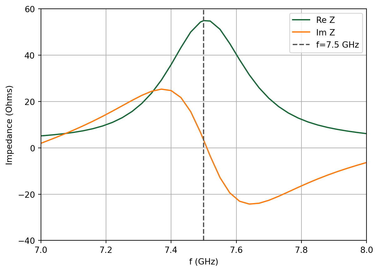

Far-field Metrics

Directivity, gain and other commonly used antenna metrics are automatically calculated when one or more radiation_monitor is defined. The user can obtain the far-field metrics by calling the get_antenna_metrics_data() method on the TCM data object.

In [26]:

# Get antenna metrics
antenna_metrics = tcm_data.get_antenna_metrics_data()

Below, we list all of the available antenna far-field metrics for the user’s reference.

In [27]:

# The available antenna metrics quantities are listed below:

# Directivity
directivity = antenna_metrics.directivity

# Radiation efficiency: efficiency accounting for material losses
radiation_efficiency = antenna_metrics.radiation_efficiency

# Gain: radiation efficiency * directivity
gain = antenna_metrics.gain

# Reflection efficiency: efficiency accounting for impedance mismatch
reflection_efficiency = antenna_metrics.reflection_efficiency

# Realized gain: reflection efficiency * gain
realized_gain = antenna_metrics.realized_gain

# Supplied power: power supplied to antenna
supplied_power = antenna_metrics.supplied_power

# Radiated power: power radiated by antenna
radiated_power = antenna_metrics.radiated_power

# Radiation intensity: radiated intensity as a function of angle
radiation_intensity = antenna_metrics.radiation_intensity

# Axial ratio: ratio of major axis to minor axis of polarization ellipse
axial_ratio = antenna_metrics.axial_ratio

# Left and right circular polarization field components
left_polarization = antenna_metrics.left_polarization
right_polarization = antenna_metrics.right_polarization

In the following sections, we will demonstrate how to plot the gain and axial ratio.

Antenna Gain

Let’s plot the gain at the first resonance (f=7.5 GHz).

In [28]:

# Plot gain in elevation plane at f=7.5 GHz

# First, extract gain data in the forward and backward directions
gain_F = gain.sel(f=freqs_target[0], phi=0, method="nearest").squeeze()
gain_B = gain.sel(f=freqs_target[0], phi=-np.pi, method="nearest").squeeze()

# Create plot
fig = plt.figure(figsize=(8, 6), tight_layout=True)
ax = fig.add_subplot(111, projection="polar")

# Plot gain in dB
ax.set_theta_direction(-1)
ax.set_theta_offset(np.pi / 2.0)
ax.plot(theta, 10 * np.log10(np.abs(gain_F)), "-b")
ax.plot(-theta, 10 * np.log10(np.abs(gain_B)), "-b")
ax.set_title("Antenna Gain (dB) in XZ plane", y=1.08)
plt.show()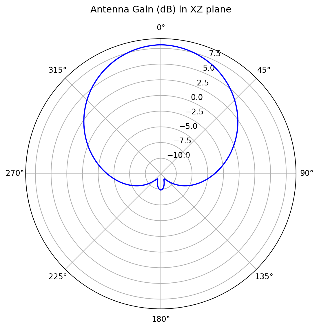

In [29]:

# Plot gain in azimuthal plane at f=7.5 GHz

# Extract gain in azimuthal plane
gain_azi = gain.sel(f=freqs_target[0], theta=np.pi / 2, method="nearest").squeeze()

# Create plot
fig = plt.figure(figsize=(8, 6), tight_layout=True)
ax = fig.add_subplot(111, projection="polar")

# Plot gain in dB
ax.plot(phi, 10 * np.log10(np.abs(gain_azi)), "-b")
ax.set_title("Antenna Gain (dB) in XY plane", y=1.08)
plt.show()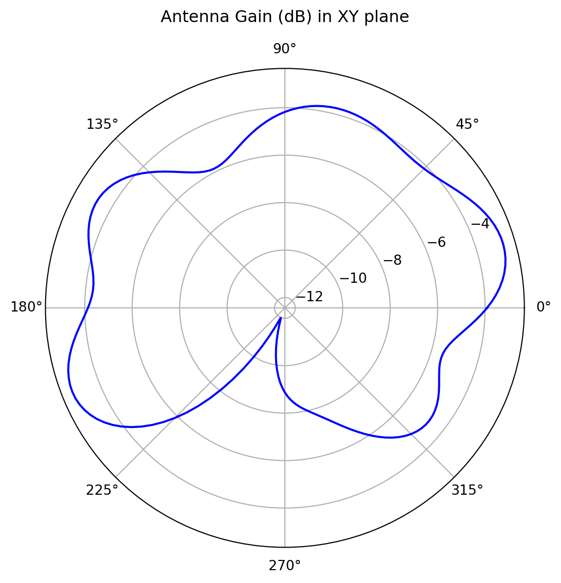

We can also create an interactive 3D plot of the gain.

In [30]:

# Rescale gain according to max and min dB values
dB_min, dB_max = (-20, 10)
G = 10 * np.log10(np.abs(gain.sel(f=7.5e9, method="nearest").squeeze()))
G_scaled = np.clip((G - dB_min) / (dB_max - dB_min), a_min=0, a_max=1)

# Build the gain-radius surface in cartesian coordinates
phi_s, theta_s = np.meshgrid(phi, theta)
X = G_scaled * np.cos(phi_s) * np.sin(theta_s)
Y = G_scaled * np.sin(phi_s) * np.sin(theta_s)
Z = G_scaled * np.cos(theta_s)

# Color the surface by gain in dB (clipped to the chosen range)
G_clipped = np.clip(G, dB_min, dB_max)

fig_3d = go.Figure(
    data=go.Surface(
        x=X,
        y=Y,
        z=Z,
        surfacecolor=G_clipped,
        cmin=dB_min,
        cmax=dB_max,
        colorscale="Jet",
        colorbar=dict(title="G (dB)"),
    )
)
fig_3d.update_layout(
    scene=dict(
        xaxis=dict(title="x", showticklabels=False, range=[-1, 1]),
        yaxis=dict(title="y", showticklabels=False, range=[-1, 1]),
        zaxis=dict(title="z", showticklabels=False, range=[-1, 1]),
        aspectmode="cube",
        camera=dict(eye=dict(x=1.6, y=1.6, z=1.2)),
    ),
    margin=dict(l=20, r=20, t=20, b=20),
    height=500,
)

fig_3d.show()

Axial Ratio

Let’s plot the axial ratio vs frequency for the main lobe (phi, theta = 0)

In [31]:

# Extract axial ratio at main lobe
axial_ratio_main_lobe = axial_ratio.sel(theta=0, phi=0, method="nearest").squeeze()

In [32]:

# Plot main lobe axial ratio vs frequency
fig, ax = plt.subplots()
ax.plot(freqs / 1e9, 20 * np.log10(axial_ratio_main_lobe))
ax.grid()
ax.set_xlabel("f (GHz)")
ax.set_ylabel("Axial ratio (dB)")
plt.show()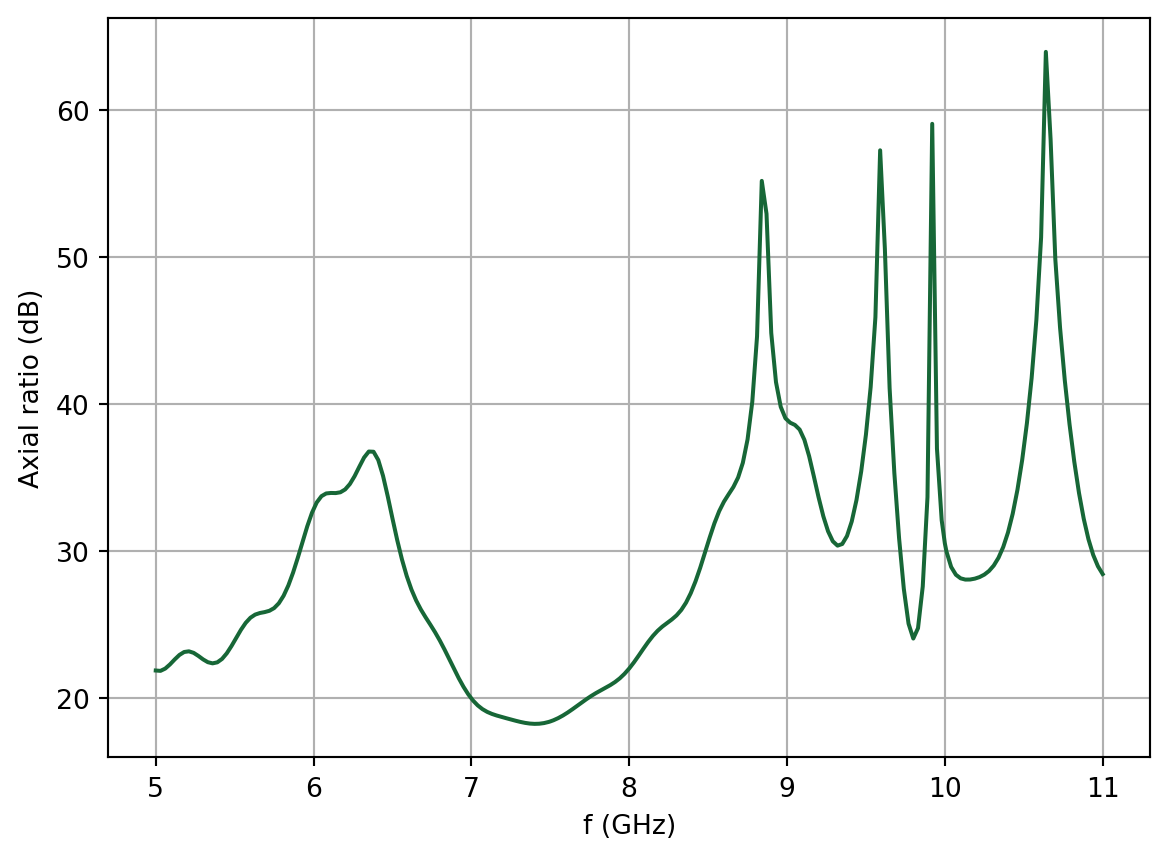

Reference

[1] Sheen, D.M., Ali, S.M., Abouzahra, M.D. and Kong, J.A., 1990. Application of the three-dimensional finite-difference time-domain method to the analysis of planar microstrip circuits. IEEE Transactions on microwave theory and techniques, 38(7), pp.849-857.