Quickstart Demonstration

On this page, we will construct a simple 3D microwave simulation with Flexcompute RF (also Flex RF) to demonstrate the typical workflow.

For a more detailed discussion, please refer to our User Guide.

We begin with the Python imports. We will also make use of third-party packages numpy and matplotlib. Basic familiarity with these packages is assumed.

# Import main flex_rf package
import flex_rf.tidy3d as rf

# Import web module for cloud job management
import flex_rf.web as web

# Import third-party math and plotting libraries
import numpy as np
import matplotlib.pyplot as plt

Next, we define the simulation frequency range and design parameters.

# Frequency
f_min, f_max = (1e9, 20e9)
f0 = (f_min + f_max)/2
freqs = np.linspace(f_min, f_max, 401)

# Geometry dimensions
mm = 1000                                       # conversion factor from default unit (microns)
Lsub, Wsub = (20 * mm, 20 * mm)                 # substrate dimensions
Hsub = 1.5 * mm                                 # substrate thickness
Hmetal = 0.035 * mm                             # metal thickness
Lpatch, Wpatch = (8 * mm, 12 * mm)              # patch dimensions
Lfeed, Wfeed = ((Lsub - Lpatch) / 2, 2.9 * mm)  # feedline size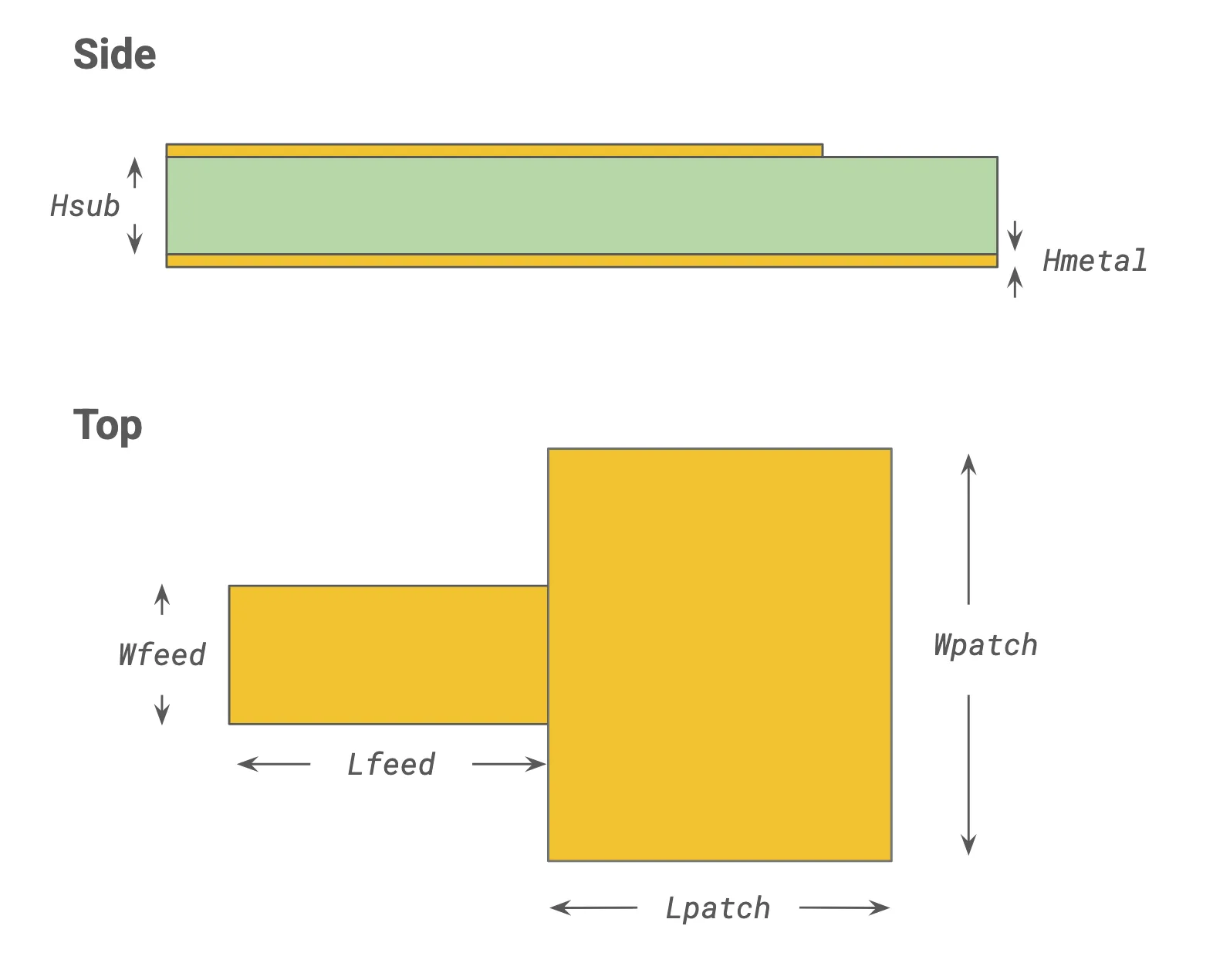

We set up the physical scene next. A physical structure is defined by the Structure object, which is composed of a geometry and a medium (material model).

# Define mediums (material models)
metal = rf.LossyMetalMedium(conductivity=58, frequency_range=(f_min, f_max))  # [S/um]
dielectric = rf.Medium(permittivity=4.3)

# Define physical structures
substrate = rf.Structure(
    geometry=rf.Box(center=(0, 0, -Hsub / 2), size=(Lsub, Wsub, Hsub)),
    medium=dielectric
)

ground = rf.Structure(
    geometry=rf.Box(center=(0, 0, -Hsub - Hmetal / 2), size=(Lsub, Wsub, Hmetal)), medium=metal
)
feed = rf.Structure(
    geometry=rf.Box(center=(-Lpatch / 2 - Lfeed / 2, 0, Hmetal / 2), size=(Lfeed, Wfeed,Hmetal)),
    medium=metal
)
patch = rf.Structure(
    geometry=rf.Box(center=(0, 0, Hmetal / 2), size=(Lpatch, Wpatch, Hmetal)),
    medium=metal
)

structure_list = [substrate, ground, feed, patch]

The patch is excited via the feed line. Excitations in Flex RF are also known as ports. We connect the end of the feed line to a LumpedPort. The default impedance of a lumped port is 50 Ohms.

# Define port
port_1 = rf.LumpedPort(
    center=(-Lsub / 2, 0, -Hsub / 2),
    size=(0, Wfeed, Hsub),
    voltage_axis=2,                    # axis of voltage drop (2 = Z-axis)
    name="port_1"
)

The simulation will automatically calculate S-parameters for all included ports. Port voltages, currents, and impedances are also available.

By default, the electric and magnetic fields are not stored. To record the fields within a specific region, we define a FieldMonitor.

# Define field monitor to record at the z=0 plane
mon_1 = rf.FieldMonitor(size=(rf.inf, rf.inf, 0), freqs=[f0], name="field (z=0)")

The simulation grid is automatically generated based on the wavelength in the dielectric medium. For RF/microwave problems, it is typically also important to resolve the field near metallic structures.

# Define layer refinement around metallic structures
layer_ref_1 = rf.LayerRefinementSpec.from_structures(structures=[feed, patch])
layer_ref_2 = rf.LayerRefinementSpec.from_structures(structures=[ground])

# Define overall grid specification (auto based on wavelength)
grid_spec = rf.GridSpec.auto(
    wavelength=rf.C_0 / f0,       # Reference wavelength for automesher
    min_steps_per_wvl=15,         # Minimum grid steps per wavelength
    layer_refinement_specs=[layer_ref_1, layer_ref_2],
)

Finally, all of the components are assembled into a base Simulation. Then, the TerminalComponentModeler object implements a port/frequency sweep around the base Simulation to obtain the full S-matrix.

# Define base simulation
sim = rf.Simulation(
    size=(30 * mm, 30 * mm, 8 * mm),
    structures=structure_list,
    monitors=[mon_1],
    grid_spec=grid_spec,
    run_time=5e-9,
    plot_length_units="mm",
)

# Define TerminalComponentModeler
tcm = rf.TerminalComponentModeler(
    simulation=sim,
    ports=[port_1],
    freqs=freqs
)

The simulation is ready to submit to the cloud.

# Send the job to the cloud and await results
tcm_data = web.run(tcm, task_name='Quickstart demo')

Once the job is completed, we can extract the S-parameters and plot them.

# Extract S-matrix
s_matrix = tcm_data.smatrix()

# Extract S11 (dB)
S11 = s_matrix.data.sel(port_in='port_1', port_out='port_1')
S11dB = 20*np.log10(np.abs(S11))

# Plot S11 (dB)
fig, ax = plt.subplots(figsize=(10, 4), tight_layout=True)
ax.plot(S11dB.f / 1e9, S11dB, label='|S11|$^2$ (dB)')
ax.legend()
ax.grid()
ax.set(xlabel="f (GHz)", ylabel="dB")
plt.show()

We can also plot the field in the included FieldMonitor.

# Get simulation data corresponding to 'port_1' excitation
sim_data = tcm_data.data['port_1']

# Plot the electric field amplitude
fig, ax = plt.subplots(figsize=(6,4), tight_layout=True)
sim_data.plot_field("field (z=0)", field_name="E", val="abs", ax=ax)
plt.show()