Edge-feed Patch Antenna

Download as:

Quarto (.qmd)

The patch antenna is a ubiquitous antenna type used in modern wireless communication systems. In this notebook, we demonstrate how to simulate a patch antenna using the Flexcompute RF solver and compute key metrics, such as return loss and antenna gain profile.

In [1]:

import matplotlib.pyplot as plt
import numpy as np
import flex_rf.tidy3d as rf
import flex_rf.web as web
import plotly.graph_objects as go
import plotly.io as pio
rf.config.logging.level = 'ERROR'

# Set plotly renderer default
pio.renderers.default = "plotly_mimetype+notebook_connected"

Setup

General Parameters

We will conduct a broadband sweep from 10 MHz to 40 GHz to scan for the resonance(s) of this patch antenna. The target operating frequency of the antenna is around 35.3 GHz.

In [2]:

# Frequency range
f_min, f_max = (0.01e9, 40e9)

# Target operating frequency
f_target = 35.3e9

# Frequency sample points (including f_target)
freqs = np.sort(np.append(np.linspace(f_min, f_max, 301), f_target))

Material and Structures

Both the substrate and conductor materials are assumed to be lossy and have constant loss parameters over the frequency range.

In [3]:

# Lossy substrate (rel. epsilon = 2.2, loss tangent = 0.0009)
med_sub = rf.FastDispersionFitter.constant_loss_tangent_model(
    2.2, 0.0009, (f_min, f_max), tolerance_rms=2e-4
)

# Lossy metal (conductivity = 58e6 S/m)
med_metal = rf.LossyMetalMedium(conductivity=58, frequency_range=(f_min, f_max))

Best weighted RMS error: 0.000152 ━━━━━━━━━━━━━━━━━━━━━━━━━━━━━━━━━ 100% 0:00:00

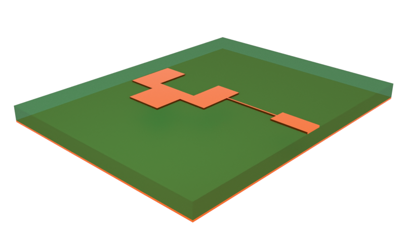
The geometry is constructed below. Note that the default length unit is microns. We introduce a scaling factor mm for convenience.

In [4]:

# Geometry parameters
mm = 1000
t = 0.02 * mm  # Metal thickness
h = 0.254 * mm  # Substrate thickness

In [5]:

# Create substrate and ground planes
str_sub = rf.Structure(
    geometry=rf.Box(center=(0, 0, -h / 2), size=(6 * mm, 10 * mm, h)), medium=med_sub
)
str_gnd = rf.Structure(
    geometry=rf.Box(center=(0, 0, -h - t / 2), size=(6 * mm, 10 * mm, t)), medium=med_metal
)

# Create feed structure
str_feed1 = rf.Structure(
    geometry=rf.Box.from_bounds(rmin=(2 * mm, -0.31 * mm, 0), rmax=(3 * mm, 0.31 * mm, t)),
    medium=med_metal,
)
str_feed2 = rf.Structure(
    geometry=rf.Box.from_bounds(rmin=(0.5 * mm, -0.05 * mm, 0), rmax=(2 * mm, 0.05 * mm, t)),
    medium=med_metal,
)

# Create antenna structure
ant_vertices = (
    np.array(
        [
            [-1.3, -2.1],
            [-0.3, -2.1],
            [-0.3, -1.1],
            [0.5, -1.1],
            [0.5, 0.6],
            [-0.19, 0.6],
            [-0.19, -0.62],
            [-1.4, -0.62],
            [-1.4, 0.6],
            [-2.1, 0.6],
            [-2.1, -1.1],
            [-1.3, -1.1],
        ]
    )
    * mm
)
str_ant = rf.Structure(
    geometry=rf.PolySlab(axis=2, slab_bounds=[0, t], vertices=ant_vertices), medium=med_metal
)

# Full structure list
str_list_full = [str_sub, str_gnd, str_feed1, str_feed2, str_ant]

Grid and Boundary

The perfectly matched layer (PML) boundary is applied by default on all external boundaries. As is standard practice for radiation problems, we also include an air buffer region around the antenna.

In [6]:

# Define simulation size with padding
padding = rf.C_0 / f_target / 4
sim_LX = 6 * mm + 2 * padding
sim_LY = 10 * mm + 2 * padding
sim_LZ = 2 * t + h + 2 * padding

The grid size in dielectric media is typically determined by the propagating wavelength. Thus, in the overall grid specification, we set the maximum grid step size to be wavelength/20.

That said, it is also important to refine the grid near the metallic structures, as they are responsible for the resonant behavior of the antenna. The LayerRefinementSpec serves this purpose. We define a function that creates LayerRefinementSpec objects in the top layer (feed structure and antenna) and bottom layer (ground plane) respectively.

Within each layer, the grid is refined in the normal direction (z) as well as around any metal corners. These are controlled by the min_steps_along_axis and corner_refinement parameters respectively.

In [7]:

# Define layer refinement on metallic structures
def create_layer_refinement(structure_list):
    """Create predefined layer refinement spec for input structure list"""
    return rf.LayerRefinementSpec.from_structures(
        structures=structure_list,
        min_steps_along_axis=2,
        corner_refinement=rf.GridRefinement(dl=0.05*mm, num_cells=2),
    )

lr1 = create_layer_refinement([str_gnd])
lr2 = create_layer_refinement([str_feed1, str_feed2, str_ant])

In [8]:

# Define grid specification
gspec = rf.GridSpec.auto(
    wavelength=rf.C_0 / f_target,
    min_steps_per_wvl=20,
    layer_refinement_specs=[lr1, lr2],
)

Excitation

The antenna is fed using a 50-ohm microstrip line. We excite the microstrip line with a lumped port of the corresponding impedance, connected to the end of the feed structure.

In [9]:

# Define lumped port excitation
LP1 = rf.LumpedPort(
    center=(3 * mm, 0, -h / 2), size=(0, 0.62 * mm, h), voltage_axis=2, impedance=50, name="LP1"
)

Monitors

We define two field monitors to visualize the near-field profile at the target resonance frequency.

In [10]:

# Define near field monitors
mon1 = rf.FieldMonitor(
    center=(0, 0, 0), size=(rf.inf, 0, rf.inf), freqs=[f_target], name="xz plane"
)
mon2 = rf.FieldMonitor(
    center=(0, 0, 0), size=(rf.inf, rf.inf, 0), freqs=[f_target], name="xy plane"
)

Far-field radiation data is calculated by the DirectivityMonitor that encloses the whole antenna structure.

In [11]:

# Define elevation and azimuthal angular observation points
# Theta is the elevation angle and defined relative to global +z axis
theta = np.linspace(0, np.pi, 91)
# Phi is the azimuthal angle and defined relative to global +x axis
phi = np.linspace(0, 2*np.pi, 181)

# The DirectivityMonitor calculates the radiation pattern using a near-to-far-field transformation
mon_radiation = rf.DirectivityMonitor(
    center=(0, 0, 0),
    size=(
        0.9 * sim_LX,
        0.9 * sim_LY,
        0.9 * sim_LZ,
    ),  # The monitor should enclose the whole structure of interest
    freqs=[f_target],
    name="radiation",
    phi=phi,
    theta=theta,
)

Simulation and TerminalComponentModeler

The base Simulation object gathers all the relevant settings so far.

In [12]:

# Define simulation object
sim = rf.Simulation(
    size=(sim_LX, sim_LY, sim_LZ),
    structures=str_list_full,
    grid_spec=gspec,
    monitors=[mon1, mon2],
    run_time=3e-9,
    shutoff=1e-7,
    plot_length_units="mm",
)

The TerminalComponentModeler (TCM) is a wrapper object that automatically runs a port sweep on the simulation using user-defined ports and constructs the full S-parameter matrix. In this case there is only 1 port. The radiation_monitors setting is where we include the previously defined DirectivityMonitor.

Note that when the minimum frequency is less than 1 GHz, we recommend setting remove_dc_component to False and increasing the run_time setting in Simulation.

In [13]:

# Define TerminalComponentModeler
tcm = rf.TerminalComponentModeler(
    simulation=sim,
    ports=[LP1],
    radiation_monitors=[mon_radiation],
    freqs=freqs,
    remove_dc_component=False,
)

Plotting

Before running, we should plot the simulation and check the grid.

In [14]:

# Visualize the simulation in 3D (ports and radiation monitor not shown)
sim.plot_3d()

In [15]:

# Plot structures and grid at z=0 and y=0 cross sections
fig, ax = plt.subplots(2, 1, figsize=(8, 10), tight_layout=True)
tcm.plot_sim(z=0, ax=ax[0], monitor_alpha=0)
sim.plot_grid(z=0, ax=ax[0])
ax[0].set_xlim(-4 * mm, 4 * mm)
ax[0].set_ylim(-6 * mm, 6 * mm)
tcm.plot_sim(y=0, ax=ax[1], monitor_alpha=0)
sim.plot_grid(y=0, ax=ax[1])
ax[1].set_xlim(-4 * mm, 4 * mm)
ax[1].set_ylim(-0.5 * mm, 0.25 * mm)
ax[1].set_aspect(3)
plt.show()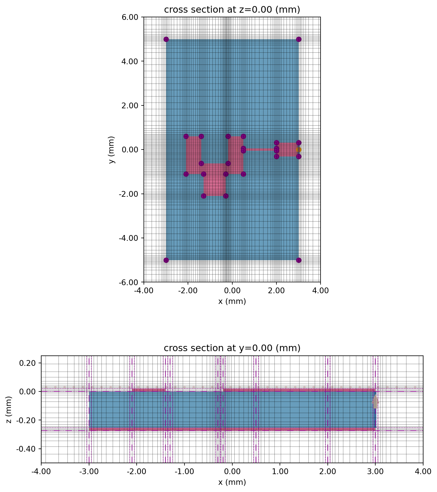

In [16]:

# Plot lumped port
fig, ax = plt.subplots(figsize=(6, 4))
tcm.plot_sim(x=3 * mm, ax=ax, monitor_alpha=0)
sim.plot_grid(x=3 * mm, ax=ax)
ax.set_xlim(-0.5 * mm, 0.5 * mm)
ax.set_ylim(-0.5 * mm, 0.3 * mm)
plt.show()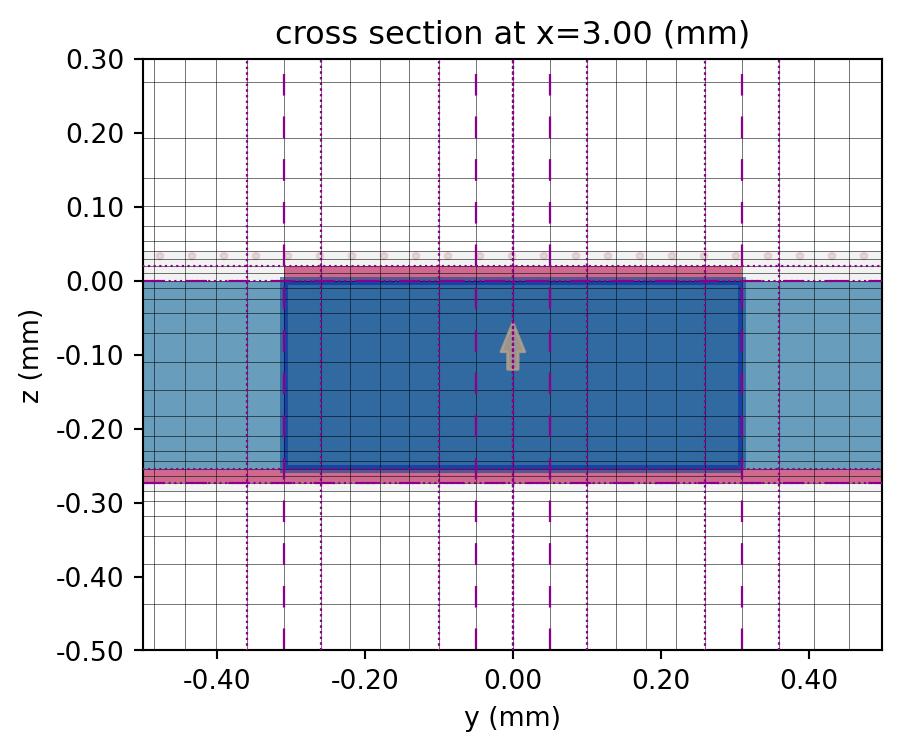

Running the Simulation

Use web.run() to send the job to the cloud and await results.

In [17]:

tcm_data = web.run(tcm, task_name="edge_feed_antenna", path='./data/edge_feed_patch_antenna.hdf5', verbose=False)

Results

S-parameter

Below, we extract and plot the simulated S11.

In [18]:

# Extract S-matrix and S11
smat = tcm_data.smatrix()
S11 = np.conjugate(smat.data.isel(port_in=0, port_out=0))

In [19]:

# Plot S11 in dB
fig, ax = plt.subplots(figsize=(8, 4), tight_layout=True)
ax.plot(freqs / 1e9, 20 * np.log10(np.abs(S11)))
ax.grid()
ax.set_xlabel("f (GHz)")
ax.set_ylabel("|S11| (dB)")
ax.set_title("Return loss")
plt.show()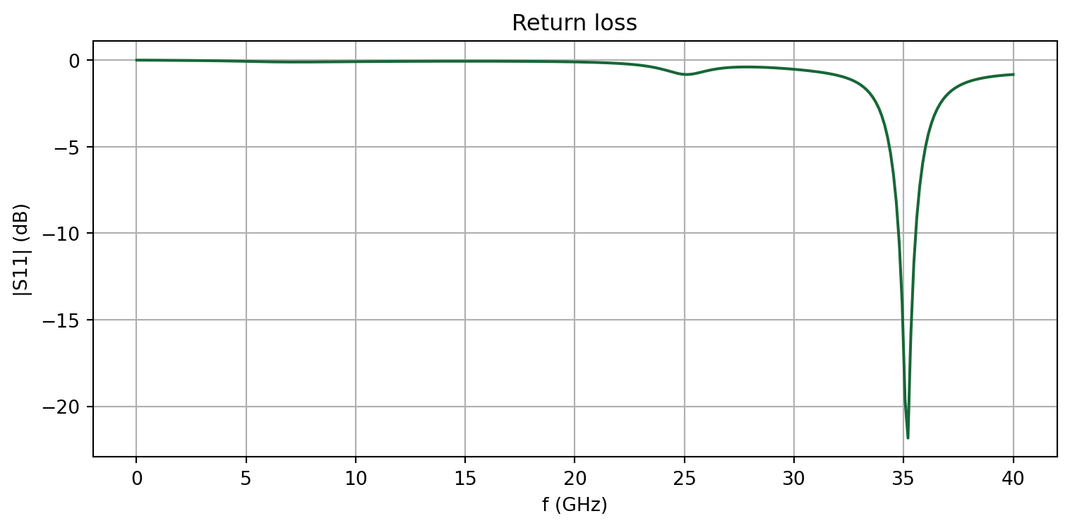

Field profiles

Data for user-defined monitors are recorded for every port in the TerminalComponentModeler. Use a specific port name as the dictionary key to access the monitor data corresponding to that port excitation.

In [20]:

# Access the simulation data for port 1 excitation
sim_data = tcm_data.data["LP1"]

We plot the field profiles at f=f_target below.

In [21]:

# Visualize near-field profiles
fig, ax = plt.subplots(1, 2, figsize=(10,3), tight_layout=True)
sim_data.plot_field(
    "xz plane", field_name="E", val="abs", scale="dB", f=f_target, ax=ax[0], vmax=0, vmin=-60
)
ax[0].set_title("Near-field magnitude (dB) in elevation plane")
ax[0].set_xlim(-6 * mm, 5 * mm)
ax[0].set_ylim(-1 * mm, 5 * mm)
sim_data.plot_field("xy plane", field_name="E", val="abs", scale="lin", f=f_target, ax=ax[1])
ax[1].set_title("Near-field magnitude (abs) in antenna plane")
ax[1].set_xlim(-3 * mm, 3.2 * mm)
ax[1].set_ylim(-2.6 * mm, 1.3 * mm)
plt.show()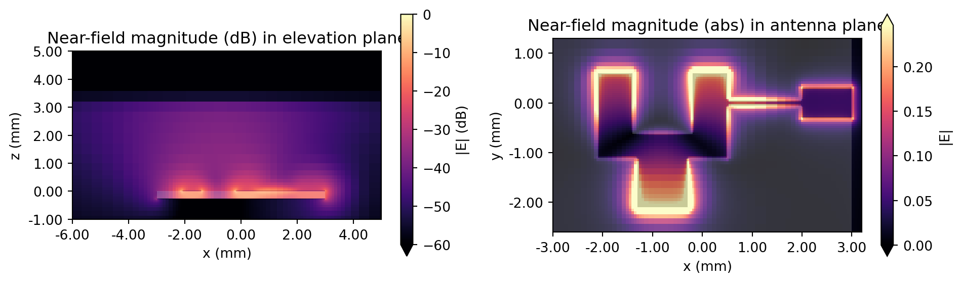

Antenna Gain

The get_antenna_metrics_data() method of the TCM data object calculates and returns common antenna metrics.

In [22]:

# Get antenna metrics from simulation data
antenna_metrics = tcm_data.get_antenna_metrics_data()

# Extract gain data
gain = antenna_metrics.gain

Below is a convenience function that collects the gain data for forward and backward directions (phi and phi-180 degrees) into a single array.

In [23]:

def get_full_elevation_plane_data(data, phi_forward, phi_backward):
    """Get full elevation plane data for given phi (azimuth) forward and backward angle"""
    # Assemble full theta (elevation angle) coordinate
    thetas = data.theta
    thetas_full = np.unique(np.append(-thetas, thetas))

    # Assemble data
    data_forward = data.sel(phi=phi_forward, method="nearest").squeeze()
    data_backward = data.sel(phi=phi_backward, method="nearest").squeeze()
    data_full = np.append(data_backward[:0:-1], data_forward)

    return thetas_full, data_full

The gain data for the elevation planes phi=0 degrees and phi=90 degrees are collected below.

In [24]:

# Get gain in the elevation plane for phi = 0 and 90 degrees
theta_elev, gain_elev = get_full_elevation_plane_data(gain, phi_forward=0, phi_backward=np.pi)
_, gain_elev_90 = get_full_elevation_plane_data(
    gain, phi_forward=np.pi / 2, phi_backward=3*np.pi / 2
)

We plot the antenna gain below.

In [25]:

# Gain comparison plot
fig, ax = plt.subplots(1, 2, figsize=(10, 8), tight_layout=True, subplot_kw={"projection": "polar"})

# Plot gain for phi =0
ax[0].plot(theta_elev, 10 * np.log10(gain_elev))
ax[0].set_title("Gain (dB) in elevation plane ($\\phi=0$ deg)", pad=30)

# Plot gain for phi = 90deg
ax[1].plot(theta_elev, 10 * np.log10(gain_elev_90))
ax[1].set_title("Gain (dB) in elevation plane ($\\phi=90$ deg)", pad=30)

for axis in ax:
    axis.set_theta_direction(-1)
    axis.set_theta_offset(np.pi / 2.0)

plt.show()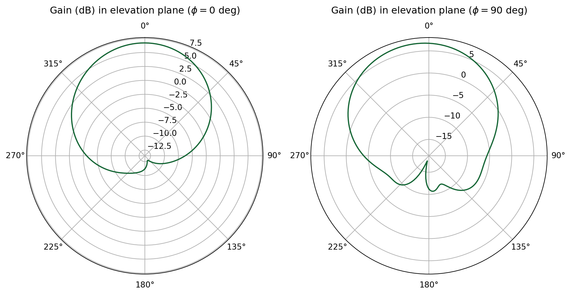

The LobeMeasurer is a post-processing tool that automatically calculates lobe measurements based on a radiation profile.

In [26]:

# Calculate radiation lobe properties
lobes = rf.LobeMeasurer(angle=theta_elev, radiation_pattern=gain_elev, apply_cyclic_extension=False)

The properties of the main lobe are reported below. Angle units are radians. In addition to the main_lobe property, users can also view lobe_measures for a summary table of all detected lobes, side_lobes for side lobe properties, and sidelobe_level.

In [27]:

# Report main lobe properties
lobes.main_lobe

direction                                                   -0.0
magnitude                                               4.696953
beamwidth                                               1.469637
beamwidth magnitude                                     2.348476
beamwidth bounds       (-0.7799961382054892, 0.6896404398825705)
FNBW                                                         NaN
FNBW bounds                                           (nan, nan)
Name: 0, dtype: object

The LobeMeasurer.plot() method automatically adds markers to indicate main lobe direction and -3 dB beamwidth. This is demonstrated below.

In [28]:

# Gain comparison plot
fig, ax = plt.subplots(figsize=(6, 6), tight_layout=True, subplot_kw={"projection": "polar"})
ax.set_theta_direction(-1)
ax.set_theta_offset(np.pi / 2.0)

# Plot gain for phi =0
ax.plot(theta_elev, 10 * np.log10(gain_elev / np.max(gain_elev)), color="black")
lobes.plot(lobe_index=0, ax=ax)
ax.set_ylim(-20, 1)
ax.set_title("Normalized gain (dB) with -3 dB beamwidth markers", pad=30)
plt.show()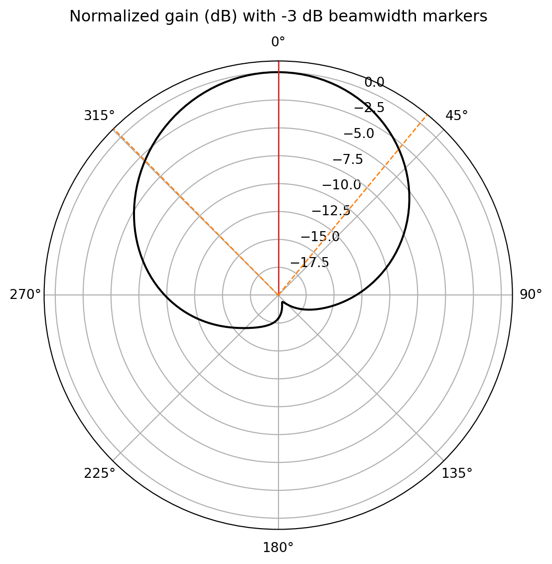

3D Radiation Pattern

In this section, we demonstrate how to plot the radiation pattern in 3D.

In [29]:

# Rescale gain according to max and min dB values
dB_min, dB_max = (-40, 25)
G = 10 * np.log10(np.abs(gain.squeeze()))
G_scaled = np.clip((G - dB_min) / (dB_max - dB_min), a_min=0, a_max=1)

# Build the gain-radius surface in cartesian coordinates
phi_s, theta_s = np.meshgrid(phi, theta)
X = G_scaled * np.cos(phi_s) * np.sin(theta_s)
Y = G_scaled * np.sin(phi_s) * np.sin(theta_s)
Z = G_scaled * np.cos(theta_s)

# Color the surface by gain in dB (clipped to the chosen range)
G_clipped = np.clip(G, dB_min, dB_max)

fig_3d = go.Figure(
    data=go.Surface(
        x=X,
        y=Y,
        z=Z,
        surfacecolor=G_clipped,
        cmin=dB_min,
        cmax=dB_max,
        colorscale="Jet",
        colorbar=dict(title="G (dB)"),
    )
)
fig_3d.update_layout(
    scene=dict(
        xaxis=dict(title="x", showticklabels=False, range=[-1, 1]),
        yaxis=dict(title="y", showticklabels=False, range=[-1, 1]),
        zaxis=dict(title="z", showticklabels=False, range=[-1, 1]),
        aspectmode="cube",
        camera=dict(eye=dict(x=1.6, y=1.6, z=1.2)),
    ),
    margin=dict(l=20, r=20, t=20, b=20),
    height=500,
)
fig_3d.show()

Reference

[1] Khan, J., Ullah, S., Ali, U., Tahir, F. A., Peter, I., & Matekovits, L. (2022). Design of a Millimeter-Wave MIMO Antenna Array for 5G Communication Terminals. Sensors, 22(7), 2768.