Geometry

A physical structure in Flexcompute RF (also Flex RF) is represented by a geometry and a medium. This page explains how to create and manipulate geometry. A variety of built-in primitives are supported, as well as boolean operations and spatial transformations. Collections of geometry objects can also be combined in geometry groups. Flex RF also has built-in interoperability with certain external file formats.

Note

The default length unit is the micrometer (um). Use conversion factors to work in other units.

# Define length conversion factors in your code
mm = 1000
mil = 25.4

# Use conversion factors to work in preferred units
a = 10*mm   # 10 millimeters
b = 8*mil   # 8 mils

Primitives

Create 1D lines, 2D planes, and 3D boxes with Box.

# Create a box by specifying center position and size
my_box1 = Box(center=(-2,0,0), size=(1,2,1))

# Create a box by specifying min/max bounds
my_box2 = Box.from_bounds(rmin=(-1,-0.5,-1), rmax=(1, 0.5,1))

# Create a 2D plane by setting size to zero in the normal direction
my_plane = Box(center=(0,0,-1), size=(5,5,0))

# Create a 1D line by setting size to zero in two dimensions
my_line = Box(center=(0,3,0), size=(5,0,0))

# Get the 2D planar faces of a box quickly using the surfaces() method
my_box_surfaces = Box.surfaces(center=(2,0,0), size=(1,1,1))
my_box_surfaces = my_box_surfaces[4:]  # keep only the planes normal to z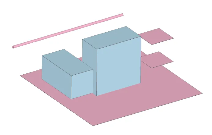

Spheres are created with the Sphere object. The Cylinder object can be used to create cylinders and conical geometry in 3D, as well as circles in 2D.

# Create a sphere
my_sphere = Sphere(center=(-2,0,0), radius=1)

# Create a cylinder
my_cylinder = Cylinder(center=(0,0,0), axis=1, radius=0.5, length=2)

# Create a conical geometry by specifying sidewall_angle (radians)
my_conical_shape = Cylinder(center=(2,0,0), axis=2, radius=0.5, length=2, sidewall_angle=np.pi/15)

# Create a circle
my_circle = Cylinder(center=(0,0,-1), axis=2, radius=5, length=0)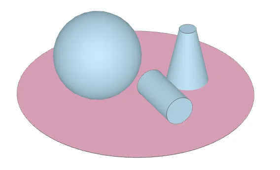

Use the PolySlab object to create custom polygons in 2D and extruded polygons in 3D.

# Specify the in-plane polygon vertices
my_vertices = np.array([(-3,0), (-1,0), (-2,1)])

# Create polyslab from vertices
my_polyslab = PolySlab(vertices=my_vertices, axis=2, slab_bounds=(0,2))

# Use the sidewall_angle attribute to create sloped polyslabs
my_vertices2 = np.array([(1, 0), (3, 0), (2.5, 1), (1.5, 1)])
my_polyslab2 = PolySlab(vertices=my_vertices2, axis=1, slab_bounds=(0,2), sidewall_angle=np.pi/20)

# Use the dilation attribute to expand/shrink each edge along its normal
my_polyslab_dilated = my_polyslab.updated_copy(dilation=0.1)   # copy and dilate by 0.1 um
my_polyslab3 = (my_polyslab_dilated - my_polyslab).translated(0, 3, 0)  # cut original shape out of dilated shape, then translate

# Use the bulge attribute to define curved edges between vertices
my_polyslab4 = my_polyslab.updated_copy(bulges=[0, 0, 1]).translated(4, 3, 0)  # copy, apply bulge and translate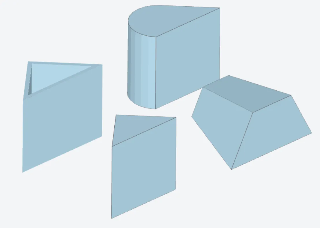

Boolean Operations

The ClipOperation object supports union, intersection, difference, and symmetric difference operations between two geometry objects.

# Difference
my_boolean1 = ClipOperation(
    operation='difference',
    geometry_a=Box(center=(-2,0,0), size=(1,1,2)),
    geometry_b=Cylinder(center=(-2,0,0), axis=2, radius=0.25, length=2)
)

# Intersection
my_boolean2 = ClipOperation(
    operation='intersection',
    geometry_a=Sphere(center=(2,0,-6), radius=6),
    geometry_b=Cylinder(center=(2,0,0), axis=2, radius=2, length=1)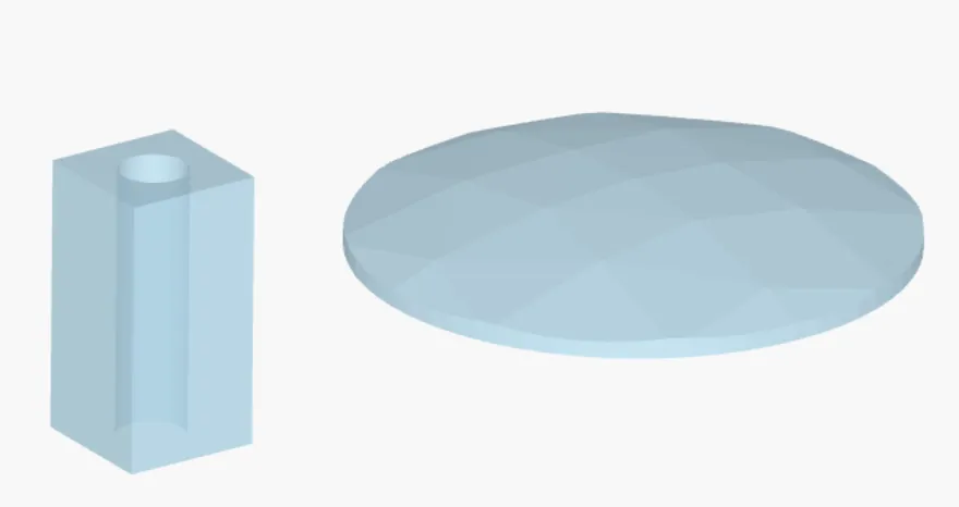
)

You can use the following binary operators as convenient shorthand for the respective operation.

Operation	Shorthand
Union	a + b
Difference	a - b
Intersection	a * b
Symmetric difference	a ^ b

# Use the binary operator as shorthand
my_box = Box(center=(-2,0,0), size=(1,1,2))
my_cylinder = Cylinder(center=(-2,0,0), axis=2, radius=0.25, length=2)
my_boolean1 = my_box - my_cylinder

Spatial Transformations and Arrays

You can use translated(), scaled(), rotated(), and reflected() with any geometry object to perform the respective transformation. A copy is returned and the original object is not modified. Multiple operations can be chained.

my_box = Box(center=(0,0,0), size=(1,1,2))

# Rotate by 30 degrees CW around Y axis
my_box_rotated = my_box.rotated(angle=np.pi/6, axis=1)

# Translate by -2 um in X, followed by reflection along X direction about origin
my_box_translated = my_box.translated(-2,0,0).reflected((1, 0, 0))

# Scale by 2x in (X, Y) directions, by 0.2x in Z
my_box_scaled = my_box.scaled(2,2,0.2)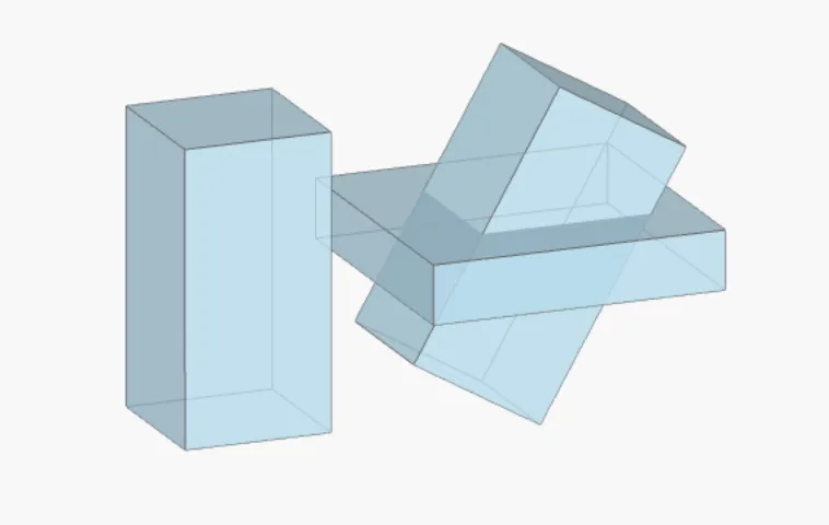

For fully general transformations, you can use the Transformed class to specify an arbitrary 4x4 transformation matrix.

# Use static methods in Transformed to generate 4D transformation matrices
mat_translation = Transformed.translation(-2, 0, 0)
mat_scaling = Transformed.scaling(1, 0.2, 1)
mat_rotation = Transformed.rotation(angle=np.pi/4, axis=1)

# Multiply matrices together to make arbitrary transformation
mat_transformation = mat_translation @ mat_rotation @ mat_scaling
my_box_transformed = Transformed(geometry=my_box, transform=mat_transformation)

To create a repeated array of geometries, use the GeometryArray object. You can also use the array() method with any geometry.

my_box = Box(size=(2,0.75,1))

# Create a linear 4 x 3 array with (3, 2) um offset in (X, Y)
offsets = [ (i*3-4, j*2-1.5, 0) for i in range(4) for j in range(3) ]
my_box_array = GeometryArray(geometry=my_box, offsets=offsets)

# Create a 24-element circular array with offset radius 10 um.
angles = np.linspace(0, 2*np.pi, 24)
offsets2 = [ ( 10*np.cos(theta), 10*np.sin(theta), 0 ) for theta in angles ]
rotations = [ Transformed.rotation(angle=theta, axis=2) for theta in angles ]
my_circular_array = my_box.array(offsets=offsets2, transforms=rotations)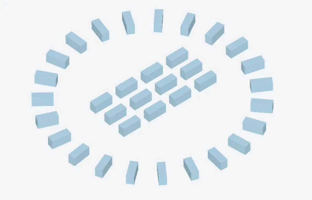

GeometryArray or for loop?

Instead of using GeometryArray, one might equivalently use a for loop to create each array element and store them in a list. The elements can then be grouped together using a GeometryGroup. The two approaches are functionally identical. However, the GeometryArray approach is more compact for serialization purposes, as the array element is stored only once, not multiple times. Thus, we recommend using GeometryArray when possible.

Geometry Groups

Instead of keeping track of multiple geometries in a list, use the GeometryGroup object to group them together.

# Group previously created geometries together
my_geom_group = GeometryGroup(geometries=[my_box, my_cylinder, my_boolean1])

A GeometryGroup is also considered a regular geometry object, and thus can be used in transformations, boolean operations, arrays, and even other geometry groups.

We recommend grouping geometries together when they share the same physical material. For instance, one can group all the copper structures in a single layer of a PCB. This will result in faster solver pre-processing, especially in scenes with large amounts of geometry.

External file formats

GDSII

The GDSII file format is commonly used in photonic integrated circuit design to specify 2D geometric shapes, labels, and other design metadata. Flex RF supports GDSII via the third-party package gdstk.

import gdstk

# Load a GDSII file
lib_loaded = gdstk.read_gds("my_gds_file.gds")

# Extract a dict of all cell names
all_cells = {c.name: c for c in lib_loaded.cells}

# Select a particular cell
cell_loaded = all_cells["MY_CELL"]

# Create a Flex RF geometry from the cell
my_gds_geometry = Geometry.from_gds(
    cell_loaded,             # cell to extrude
    gds_layer=0,             # layer number from external GDS
    gds_dtype=0,             # layer dtype from external GDS
    axis=2,                  # extrusion axis
    slab_bounds=(-4, 0),     # extrusion bounds
)

STL

The TriangleMesh object represents a tessellated geometry and stores vertex and face information.

# Create a TriangleMesh using vertex and face info
vertices = np.array([[0, 0, 0], [1, 0, 0], [0, 1, 0], [0, 0, 1]])
faces = np.array([[1, 2, 3], [0, 3, 2], [0, 1, 3], [0, 2, 1]])
my_trimesh_geom = TriangleMesh.from_vertices_faces(vertices, faces)

To import an external STL file, use the from_stl() method.

# Import an external STL
my_imported_geometry = TriangleMesh.from_stl(
    filename='my_stl_file.stl',
    scale=1000,          # Scaling for triangle coordinates. Default 1 = micron, 1000 = mm, etc.
    origin=(500, 0, 0)   # Translate origin of imported geometry. Applied after scale.
)

Miscellaneous

Here are some miscellaneous tips and tricks for working with geometry.

Use the bounds and bounding_box properties of any geometry to get its bounds. This is useful for aligning and positioning geometry relative to one another.

# Get bounds (min, max vector along each axis)
bmin, bmax = my_geometry.bounds

# Get bounding box (returns a Box object)
bbox = my_geometry.bounding_box

Use the plot() method with any geometry to make a 2D cross-section plot.

# Plot a cross section of the geometry at z=10 um
my_geometry.plot(z=10)