Tidy3D Electromagnetic Solver#

Tidy3D is a software package for solving extremely large electrodynamics problems using the finite-difference time-domain (FDTD) method. It can be controlled through either an open source python package or a web-based graphical user interface.
If you’d rather skip installation and run an example in one of our web-hosted notebooks, click here.
1. Set up Tidy3D#
Install the python library tidy3d for creating, managing, and postprocessing simulations with
pip install tidy3d
Next, configure your tidy3d package with the API key from your account.
tidy3d configure
And enter your API key when prompted.
For more detailed installation instructions, see this page.
2. Run a Simulation#
Start running simulations with just a few lines of code. Run this sample code to simulate a 3D dielectric box in Tidy3D and plot the corresponding field pattern.
# !pip install tidy3d # if needed, install tidy3d in a notebook by uncommenting this line
# import the tidy3d package and configure it with your API key
import numpy as np
import tidy3d as td
import tidy3d.web as web
# web.configure("YOUR API KEY") # if authentication needed, uncomment this line and paste your API key here
# set up global parameters of simulation ( speed of light / wavelength in micron )
freq0 = td.C_0 / 0.75
# create structure - a box centered at 0, 0, 0 with a size of 1.5 micron and permittivity of 2
square = td.Structure(
geometry=td.Box(center=(0, 0, 0), size=(1.5, 1.5, 1.5)),
medium=td.Medium(permittivity=2.0)
)
# create source - A point dipole source with frequency freq0 on the left side of the domain
source = td.PointDipole(
center=(-1.5, 0, 0),
source_time=td.GaussianPulse(freq0=freq0, fwidth=freq0 / 10.0),
polarization="Ey",
)
# create monitor - Measures electromagnetic fields within the entire domain at z=0
monitor = td.FieldMonitor(
size=(td.inf, td.inf, 0),
freqs=[freq0],
name="fields",
colocate=True,
)
# Initialize simulation - Combine all objects together into a single specification to run
sim = td.Simulation(
size=(4, 3, 3),
grid_spec=td.GridSpec.auto(min_steps_per_wvl=25),
structures=[square],
sources=[source],
monitors=[monitor],
run_time=120/freq0,
)
print(f"simulation grid is shaped {sim.grid.num_cells} for {int(np.prod(sim.grid.num_cells)/1e6)} million cells.")
# run simulation through the cloud and plot the field data computed by the solver and stored in the monitor
data = td.web.run(sim, task_name="quickstart", path="data/data.hdf5", verbose=True)
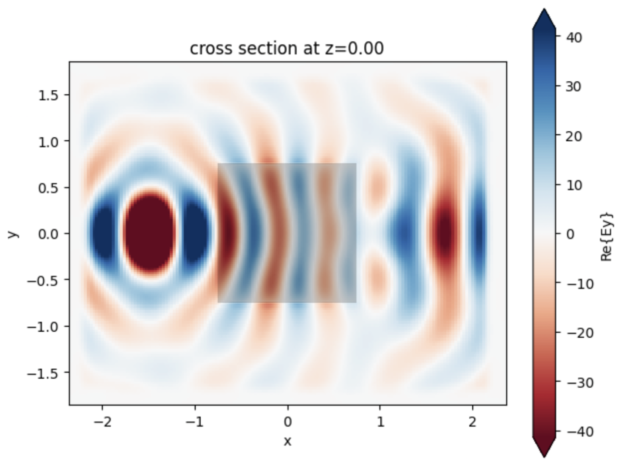
ax = data.plot_field("fields", "Ey", z=0)
This will produce the following plot, which visualizes the electromagnetic fields on the central plane.
3. Analyze Results#
Postprocess simulation data using the same python session, or
View the results of this simulation on our web-based graphical user interface.
4. Learn More#
- Installation 👋
- Lectures 📖
- Example Library 📚
- How do I … 👀
- FAQ 🔎
- What is Tidy3D?
- How can I install the Python client of Tidy3d?
- Can I do a free trial to evaluate the capabilities of Tidy3D before purchasing it?
- Can I get a discount as a student or teacher?
- What are the advantages of Tidy3D compared to traditional EM simulators?
- How do I run a simulation and access the results?
- How is using Tidy3D billed?
- Do I have to know Python programming to use Tidy3D?
- How to submit a simulation in Python to the server?
- What are the units used in the simulation?
- How are results normalized?
- What source bandwidth should I use for my simulation?
- How do I include material dispersion?
- Can I import my own tabulated material data?
- Why did my simulation finish early?
- Should I make sure that fields have fully decayed by the end of the simulation?
- Why can I not change Tidy3D instances after they are created?
- What do I need to know about the numerical grid?
- How fine of a grid or mesh does my simulation need? How to choose grid spec?
- How to use the automatic nonuniform meshing? What steps per wavelength will be sufficient?
- How to run a 2D simulation in Tidy3D?
- Can I have structures larger than the simulation domain?
- Why is a simulation diverging?
- How to troubleshoot a diverged FDTD simulation
- API 💻
- Development Guide 🛠️
- Changelog ⏪
- Unreleased
- 2.6.0rc1 - 2024-01-11
- 2.5.1 - 2024-01-08
- 2.5.0 - 2023-12-13
- 2.4.3 - 2023-10-16
- 2.4.2 - 2023-9-28
- 2.4.1 - 2023-9-20
- 2.4.0 - 2023-9-11
- 2.3.3 - 2023-07-28
- 2.3.2 - 2023-7-21
- 2.3.1 - 2023-7-14
- 2.3.0 - 2023-6-30
- 2.2.3 - 2023-6-15
- 2.2.2 - 2023-5-25
- 2.2.1 - 2023-5-23
- 2.2.0 - 2023-5-22
- 2.1.1 - 2023-4-25
- 2.1.0 - 2023-4-18
- 2.0.3 - 2023-4-11
- 2.0.2 - 2023-4-3
- 2.0.1 - 2023-3-31
- 1.10.0 - 2023-3-28
- 1.9.3 - 2023-3-08
- 1.9.2 - 2023-3-08
- 1.9.1 - 2023-3-06
- 1.9.0 - 2023-3-01
- 1.8.4 - 2023-2-13
- 1.8.3 - 2023-1-26
- 1.8.2 - 2023-1-12
- 1.8.1 - 2022-12-30
- 1.8.0 - 2022-12-14
- 1.7.1 - 2022-10-10
- 1.7.0 - 2022-10-03
- 1.6.3 - 2022-9-13
- 1.6.2 - 2022-9-6
- 1.6.1 - 2022-8-31
- 1.6.0 - 2022-8-29
- 1.5.0 - 2022-7-21
- 1.4.1 - 2022-6-13
- 1.4.0 - 2022-6-3
- 1.3.3 - 2022-5-18
- 1.3.2 - 2022-4-30
- 1.3.1 - 2022-4-29
- 1.3.0 - 2022-4-26
- 1.2.2 - 2022-4-16
- 1.2.1 - 2022-3-30
- 1.2.0 - 2022-3-28
- 1.1.1 - 2022-3-2
- 1.1.0 - 2022-3-1
- 1.0.2 - 2022-2-24
- 1.0.1 - 2022-2-16
- 1.0.0 - 2022-1-31
- 0.2.0 - 2022-1-29
- 0.1.1 - 2021-11-09
- 0.1.0 - 2021-10-21
- Alpha Release Changes
- About our Solver