tidy3d.ModeSource

class ModeSource

Bases: DirectionalSource, PlanarSource, BroadbandSource

Injects current source to excite modal profile on finite extent plane.

Parameters:

• name (Attribute: name) –

  Type	Optional[str]
  Default	= None
  Description	Optional name for the source.

• center (Attribute: center) –

  Type	Tuple[float, float, float]
  Default	= (0.0, 0.0, 0.0)
  Units	um
  Description	Center of object in x, y, and z.

• size (Attribute: size) –

  Type	Tuple[NonNegativeFloat, NonNegativeFloat, NonNegativeFloat]
  Default
  Units	um
  Description	Size in x, y, and z directions.

• source_time (Attribute: source_time) –

  Type	Union[GaussianPulse, ContinuousWave, CustomSourceTime]
  Default
  Description	Specification of the source time-dependence.

• num_freqs (Attribute: num_freqs) –

  Type	ConstrainedIntValue
  Default	= 1
  Description	Number of points used to approximate the frequency dependence of injected field. A Chebyshev interpolation is used, thus, only a small number of points, i.e., less than 20, is typically sufficient to obtain converged results.

• direction (Attribute: direction) –

  Type	Literal[‘+’, ‘-‘]
  Default
  Description	Specifies propagation in the positive or negative direction of the injection axis.

• mode_spec (Attribute: mode_spec) –

  Type	ModeSpec
  Default	= ModeSpec(num_modes1, target_neffNone, num_pml(0,, 0), filter_polNone, angle_theta0.0, angle_phi0.0, precision’single’, bend_radiusNone, bend_axisNone, track_freq’central’, group_index_stepFalse, type’ModeSpec’)
  Description	Parameters to feed to mode solver which determine modes measured by monitor.

• mode_index (Attribute: mode_index) –

  Type	NonNegativeInt
  Default	= 0
  Description	Index into the collection of modes returned by mode solver. Specifies which mode to inject using this source. If larger than mode_spec.num_modes, num_modes in the solver will be set to mode_index + 1.

Notes

Using this mode source, it is possible selectively excite one of the guided modes of a waveguide. This can be computed in our eigenmode solver tidy3d.plugins.mode.ModeSolver and implement the mode simulation in FDTD.

Mode sources are normalized to inject exactly 1W of power at the central frequency.

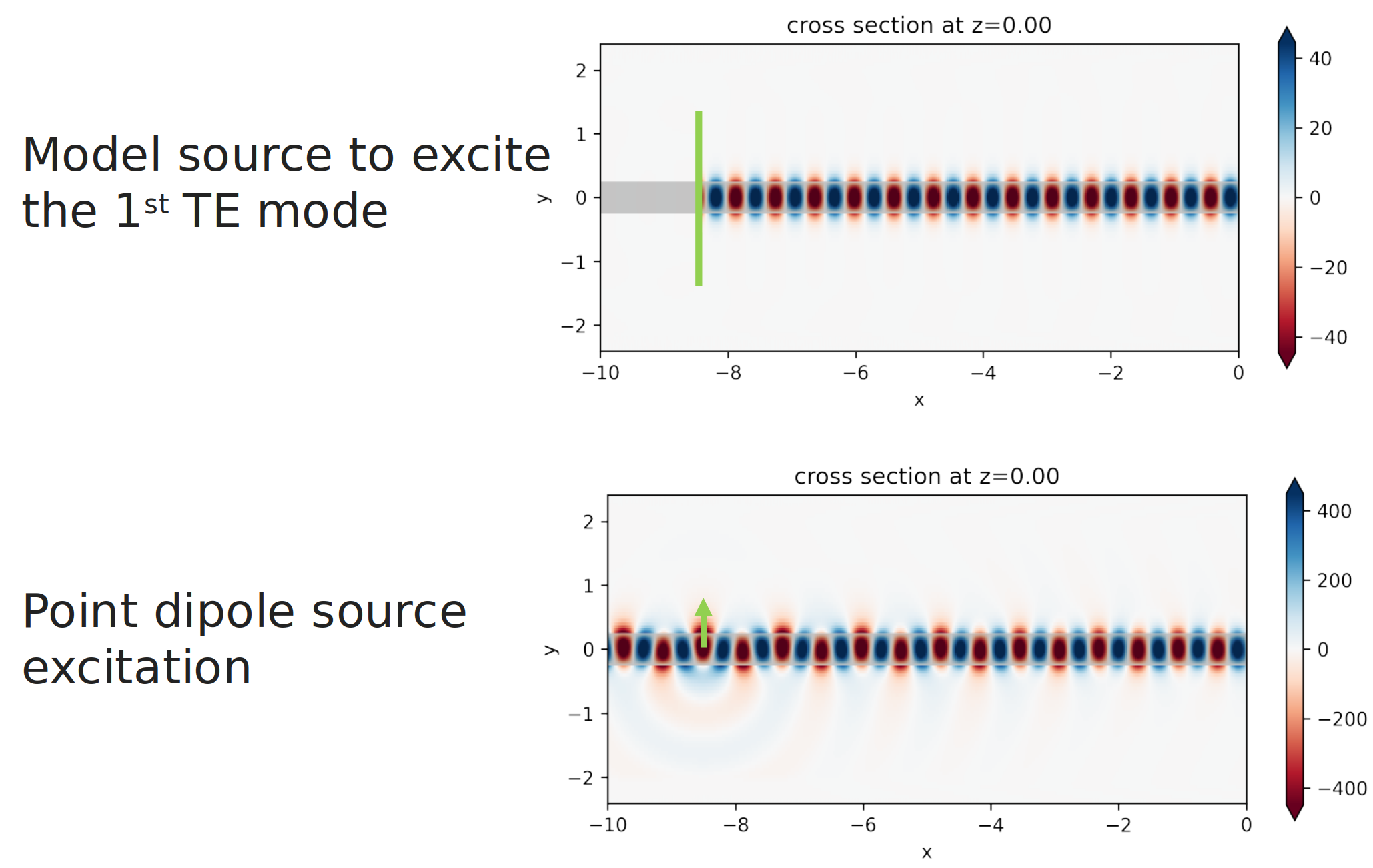
The modal source allows you to do directional excitation. Illustrated by the image below, the field is perfectly launched to the right of the source and there’s zero field to the left of the source. Now you can contrast the behavior of the modal source with that of a dipole source. If you just put a dipole into the waveguide, well, you see quite a bit different in the field distribution. First of all, the dipole source is not directional launching. It launches waves in both directions. The second is that the polarization of the dipole is set to selectively excite a TE mode. But it takes some propagation distance before the mode settles into a perfect TE mode profile. During this process, there is radiation into the substrate.

Example

>>> pulse = GaussianPulse(freq0=200e12, fwidth=20e12)
>>> mode_spec = ModeSpec(target_neff=2.)
>>> mode_source = ModeSource(
...     size=(10,10,0),
...     source_time=pulse,
...     mode_spec=mode_spec,
...     mode_index=1,
...     direction='-')

See also

tidy3d.plugins.mode.ModeSolver:

Interface for solving electromagnetic eigenmodes in a 2D plane with translational invariance in the third dimension.

Notebooks:

• Waveguide Y junction

• 90 degree optical hybrid

Lectures:

• Prelude to Integrated Photonics Simulation: Mode Injection

Attributes

angle_phi	Azimuth angle of propagation.
angle_theta	Polar angle of propagation.

Methods

mode_spec

mode_index

property angle_theta

Polar angle of propagation.

property angle_phi

Azimuth angle of propagation.

__hash__()

Hash method.