7.2. Non-Dimensionalization and Integrated Loads Post-Processing in Flow360#

7.2.1. Introduction#

The main purpose of this tutorial is to provide a hands-on example for nondimensional inputs and outputs in Flow360. The tutorial includes running CFD cases with different \(L_{gridUnit}\) values, showing how the different mesh scaling affects the output and how to convert the output to dimensional values. Additionally conventions with respect to forces in body/stability axes are also presented. Three different cases are used for this tutorial:

  • the CRM wing-body used during the 7th Drag Prediction Workshop

  • the XV-15 rotor blade using a time-accurate solution

  • the XV-15 rotor blade using a blade element theory (BET) disk solution

Note

Any value presented here in symbolic format (for example \(A_{ref}\)) refers to a dimensional value, whereas any value written in code format (for example geometry->refArea) refers to a nondimensional value that is an input to the Flow360.json file.

7.2.2. Flow360 json file input calculations#

Firstly, the Flow360 json file input calculations are demonstrated for three different cases using different \(L_{gridUnit}\) values. The \(L_{gridUnit}\) value is defined as the physical length represented by unit length in the given mesh file. Since the Flow360 solver is nondimensional, the \(L_{gridUnit}\) value is used to scale all length inputs. This allows the user to construct a mesh in any desired unit. Typical units are: meters, millimeters, feet, inches or reference chord lengths. However, care must be taken when calculating input values such as Reynolds number or rotational speed, omega, to ensure that the same solution is obtained across different mesh scales. The \(L_{gridUnit}\) values for commonly used mesh units are shown in Table 7.2.1

Table 7.2.1 \(L_{gridUnit}\) values for commonly used mesh units.#

Mesh Unit Length

\(L_{gridUnit}\)

metres [m]

1.0 m

millimetres [mm]

1 mm = 0.001 m

feet [ft]

1 ft = 0.3048 m

inches [in]

1 in = 0.0254 m

unit chords [c=1.0]

1 c_ref = (value of c_ref in metres)

Typically for CFD studies, the user will either be given a Reynolds number directly from experimental data, or the value will have to be calculated. The Reynolds number can be calculated using the following equation, with the \(L_\text{ref}\) taking the value of the experimental reference legnth in grid units and \(L_{gridUnit}\) value taken from the table above. The experimental Reynolds number can be obtained using the following calculator

(7.2.1)#\[Re_\text{CFD} = \frac{\rho_\infty U_\text{ref} \text{L}_\text{gridUnit}}{\mu_\infty} = Re_\text{EXP} \cdot \frac{{L}_\text{gridUnit}}{\text{L}_\text{ref}}\]

7.2.2.1. CRM Wing-Body#

The CRM Wing-Body configuration has been used for the 7th Drag Prediction Workshop. The nominal flow conditions quoted on the 7th Drag Prediction Workshop website are a freestream Mach number of 0.85 and Reynolds number of \(20 \times 10^6\) based on the mean aerodynamic chord (MAC) of 275.8 inches (7.00532 meters). For this tutorial the CRM is simulated at an angle of attack of 3 degrees using the tiny grid from JAXA available here along with the Flow360Mesh.json file also available. Grids of other resolutions are available here. The simulated grid is scaled to a unit chord of 1.0. To demonstrate the nondimensionalization conventions in Flow360, the CRM is scaled to five different grid units as shown in Fig. 7.2.1.

../../_images/CRM_MAC.png

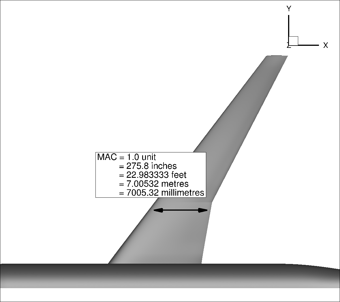
Fig. 7.2.1 CRM geometry scaled to different geometry and mesh units#

The calculation of the required inputs for the Flow360 json file, including the Reynolds number (using Eq.(7.2.1)), Flow360.json reference length (geometry->momentLength) and area (geometry->refArea) as well as the Mach number is presented in Table 7.2.2. The Flow360.json reference length is the nondimensional CRM wing MAC whereas the reference area is the nondimensional CRM wing area, with the dimensional values available here

Table 7.2.2 Solver inputs nondimensionalization for the CRM wing-body.#

MAC Unit

Unit Chord

Inches

Feet

Metres

Millimetres

\(L_{gridUnit}\)

\(1.0 c =\) \(7.00532m\)

\(1in =\) \(0.0254m\)

\(1ft =\) \(0.3048m\)

\(1m\)

\(1mm =\) \(0.001m\)

Reynolds

\(Re_\text{CFD} =\) \(20 \times 10^6 \cdot\) \(\frac{1c}{1c}=\)\(20 \times 10^6 \cdot\) \(\frac{7.00532m}{7.00532m}=\) \(20 \times 10^6\)

\(Re_\text{CFD} =\) \(20 \times 10^6 \cdot\) \(\frac{1 in}{275.8 in}=\) \(20 \times 10^6 \cdot\) \(\frac{0.0254m}{7.00532m}=\) \(72516.316\)

\(Re_\text{CFD} =\) \(20 \times 10^6 \cdot\) \(\frac{1ft}{22.98333ft}=\) \(20 \times 10^6 \cdot\) \(\frac{0.3048m}{7.00532m}=\) \(870195.794\)

\(Re_\text{CFD} =\) \(20 \times 10^6 \cdot\) \(\frac{1m}{7.00532m}=\) \(2.854973 \times 10^6\)

\(Re_\text{CFD} =\) \(20 \times 10^6 \cdot\) \(\frac{1mm}{7005.32mm}=\) \(20 \times 10^6 \cdot\) \(\frac{0.001m}{7.00532m}=\) \(2854.9731\)

geometry->momentLength

\(1.0\)

\(275.8\)

\(22.98333\)

\(7.00532\)

\(7005.32\)

geometry->refArea

\(3.909255\)

\(297360\)

\(2065\)

\(191.844778\)

\(191.844 \times 10^6\)

Mach:

0.85

0.85

0.85

0.85

0.85

The CFD calculation Reynolds number depends on the units used in the mesh due to the presence of a length component in the Reynolds number definition as seen in Eq.(7.2.1). The Flow360.json reference length (geometry->momentLength) and area (geometry->refArea) can be any value but will typically be the wing MAC and wing area nondimensionalized by \(L_{gridUnit}\) and \(L_{gridUnit}^2\) respectively. These are used to output nondimensional force and moment coefficients. The Mach number is consistent between different mesh scales. If it is unknown then it can be calculated by dividing the freestream inflow velocity with the freestream speed of sound. An example Flow360.json file is available with the mesh scaled to a unit chord of 1.0.

7.2.2.2. XV-15 Time-accurate and BET Disk#

The second example is the XV-15 rotor blade in both time-accurate and BET disk configurations. The reference data used in this example is available in this paper. Here the key parameters are the blade tip Mach number of 0.69, Reynolds number of \(4.95 \times 10^6\) based on a reference chord of 14 inches (0.3556m). The rotor radius is also required for input data and is equal to 150 inches (3.81m). The main difference between the steady-wing case and a rotor case is the need to calculate the nondimensional rotational speed, omega, as well as the time step size for the time-accurate calculation. For this tutorial we simulate the XV-15 rotor blade in hover at a collective of 10 degrees. For the time-accurate simulation a coarse grid (and Flow360Mesh.json file) is used from the time-accurate sliding interface XV-15 tutorial, whereas the coarse grid (and Flow360Mesh.json file) from blade element theory (BET) case study is used for the BET demonstration. The values used for meshes across five different units are shown in Fig. 7.2.2.

../../_images/XV15GridUnits.png

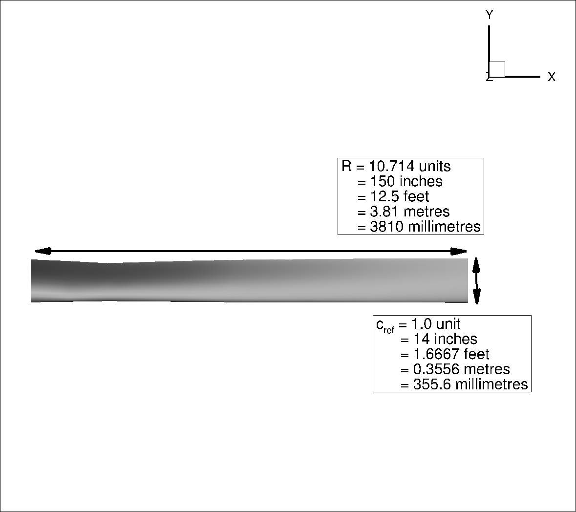
Fig. 7.2.2 XV-15 geometry scaled to different geometry and mesh units#

The calculation of the required inputs for the Flow360 json file, including the Reynolds number, Flow360.json reference length (geometry->momentLength) and area (geometry->refArea) as well as the Mach number (Mach) is presented in Table 7.2.3. Here, the reference length (geometry->momentLength) is the rotor radius nondimensionalized by the \(L_{gridUnit}\), whereas the reference area (geometry->refArea) is the rotor disk area nondimensionalized by \(L_{gridUnit}^2\) which is typical for rotor calculations. Additionally, calculations are also shown for the nondimensional omega and the time-step size equivalent to 1 degree of rotation per time step, following the conventions of Flow360. The BET disk input explicitly requires the rotor radius as an input, whereas only the time-accurate simulation requires a time step input. To calculate the nondimensional omega the following equation is used:

(7.2.2)#\[\begin{split}\omega_\text{CFD} = \Omega_\text{DIM} \cdot \frac{\text{L}_\text{gridUnit}}{C_{\infty}} = \frac{U_\text{tip}}{R} \cdot \frac{\text{L}_\text{gridUnit}}{C_{\infty}} = \\ \frac{M_\text{tip}\cdot C_{\infty}}{R} \cdot \frac{\text{L}_\text{gridUnit}}{C_{\infty}}= \frac{M_\text{tip}}{R} \cdot \text{L}_\text{gridUnit}\end{split}\]

The time step is nondimensionalized using the \(L_{gridUnit}\) value and freestream speed of sound. To obtain the time step for one degree of rotation, the rotor rotational speed is used as follows:

(7.2.3)#\[\begin{split}t_\text{CFD} = t_\text{DIM} \text{(per degree)} \cdot \frac{C_{\infty}}{\text{L}_\text{gridUnit}} = \frac{2 \pi R}{U_\text{tip}} \cdot \frac{1}{360} \cdot \frac{C_{\infty}}{\text{L}_\text{gridUnit}} = \\ \frac{2 \pi R}{M_\text{tip} \cdot C_{\infty}} \cdot \frac{1}{360} \cdot \frac{C_{\infty}}{\text{L}_\text{gridUnit}} = \frac{R}{M_\text{tip}} \cdot \frac{1}{{\text{L}_\text{gridUnit}}} \cdot \frac{\pi}{180} = \frac{1}{\omega_\text{CFD}} \cdot \frac{\pi}{180}\end{split}\]

For the XV-15 example, once again the CFD Reynolds input depends on the mesh units. For rotor calculations, the dimensional rotor radius and rotor disk area are scaled by the \(L_{gridUnit}\) and \(L_{gridUnit}^2\) to obtain the nondimensional reference length (geometry->momentLength) and area (geometry->refArea) respectively. The input Mach number (Mach) is the freestream Mach number and is zero in this case, but a reference blade tip Mach number (MachRef) of 0.69 is used for scaling forces and moments. In this case, the nondimensional omega and time step size also depend on the mesh unit. For time marching rotor solutions, the simulation is typically initialized using a 1st order solution to establish the flowfield, and then continued using the 2nd order solver (see Knowledge Base). The 1st order initial solution Flow360.json and 2nd order solution Flow360.json files are available, with meters used as the mesh unit. For the BET simulation, an example Flow360.json file is also available, with inches used as the mesh unit.

Table 7.2.3 Solver inputs nondimensionalization for the XV-15 rotor blade.#

MAC Unit

Unit Chord

Inches

Feet

Metres

Millimetres

\(L_{gridUnit}\)

\(1.0 c =\) \(0.3556m\)

\(1 in =\) \(0.0254m\)

\(1ft =\) \(0.3048m\)

\(1m\)

\(1mm =\) \(0.001m\)

Reynolds (based on \(c_{ref}\))

\(Re_\text{CFD} =\) \(4.95 \times 10^6 \cdot\) \(\frac{1c}{1c}=\) \(4.95 \times 10^6 \cdot\) \(\frac{0.3556m}{0.3556m}=\) \(4.95 \times 10^6\)

\(Re_\text{CFD} =\) \(4.95 \times 10^6 \cdot\) \(\frac{1 in}{14 in}=\) \(4.95 \times 10^6 \cdot\) \(\frac{0.0254m}{0.3556m}=\) \(353517\)

\(Re_\text{CFD} =\) \(4.95 \times 10^6 \cdot\) \(\frac{1ft}{1.6667ft}=\) \(4.95 \times 10^6 \cdot\) \(\frac{0.3048m}{0.3556m}=\) \(4.243 \times 10^6\)

\(Re_\text{CFD} =\) \(4.95 \times 10^6 \cdot\) \(\frac{1m}{0.3556m}=\) \(13.92 \times 10^6\)

\(Re_\text{CFD} =\) \(4.95 \times 10^6 \cdot\) \(\frac{1mm}{355.6mm}=\) \(4.95 \times 10^6 \cdot\) \(\frac{0.001m}{0.3556m}=\) \(13920.135\)

geometry->momentLength

\(10.714\)

\(150\)

\(12.5\)

\(3.81\)

\(3810\)

geometry->refArea

\(360.623\)

\(70685.835\)

\(490.874\)

\(45.6037\)

\(45.6037 \times 10^6\)

Mach

0.0

0.0

0.0

0.0

0.0

MachRef

0.69

0.69

0.69

0.69

0.69

omega

\(\omega_{CFD}=\) \(\frac{M_\text{tip}}{R}\) \(\cdot\text{L}_\text{gridUnit}=\) \(\frac{0.69}{10.714c}\) \(\cdot {1c}=\) \(0.064401\)

\(\omega_{CFD}=\) \(\frac{M_\text{tip}}{R}\) \(\cdot \text{L}_\text{gridUnit}=\) \(\frac{0.69}{150 in}\) \(\cdot {1 in}=\) \(0.0046\)

\(\omega_{CFD}=\) \(\frac{M_\text{tip}}{R}\) \(\cdot \text{L}_\text{gridUnit}=\) \(\frac{0.69}{12.5ft}\) \(\cdot {1ft}=\) \(0.0552\)

\(\omega_{CFD}=\) \(\frac{M_\text{tip}}{R}\) \(\cdot \text{L}_\text{gridUnit}=\) \(\frac{0.69}{3.81m}\) \(\cdot {1m}=\) \(0.1811\)

\(\omega_{CFD}=\) \(\frac{M_\text{tip}}{R}\) \(\cdot \text{L}_\text{gridUnit}=\) \(\frac{0.69}{3810mm}\) \(\cdot {1mm}=\) \(0.0001811\)

Time step per 1 degree

\(t_\text{CFD}=\) \(\frac{1}{\omega_\text{CFD}} \cdot \frac{\pi}{180}=\) \(\frac{1}{0.064401}\) \(\cdot \frac{\pi}{180}=\) \(0.271010\)

\(t_\text{CFD}=\) \(\frac{1}{\omega_\text{CFD}} \cdot \frac{\pi}{180}=\) \(\frac{1}{0.0046}\) \(\cdot \frac{\pi}{180}=\) \(3.794194\)

\(t_\text{CFD}=\) \(\frac{1}{\omega_\text{CFD}} \cdot \frac{\pi}{180}=\) \(\frac{1}{0.0552}\) \(\cdot \frac{\pi}{180}=\) \(0.316183\)

\(t_\text{CFD}=\) \(\frac{1}{\omega_\text{CFD}} \cdot \frac{\pi}{180}=\) \(\frac{1}{0.1811}\) \(\cdot \frac{\pi}{180}=\) \(0.096374\)

\(t_\text{CFD}=\) \(\frac{1}{\omega_\text{CFD}} \cdot \frac{\pi}{180}=\) \(\frac{1}{0.0001811}\) \(\cdot \frac{\pi}{180}=\) \(96.37379\)

7.2.3. Force and Moments Output Conventions#

For the steady CRM wing-body and time-marching XV15 rotor calculations, the forces and moments are output in nondimensional coefficients independent of the mesh unit. The total forces for all non-slip walls present in the calculation are stored in total_forces_v2.csv, whereas the forces on the individual non-slip walls are stored in surface_forces_v2.csv. For the BET calculation, the forces are also given in nondimensional form, but their values are scaled differently and are dependent on the mesh units used. The forces are stored in bet_forces_v2.csv. Firstly, the forces convention is presented for the steady CRM wing-body case and time-marching XV-15 rotor case, and following, the conventions for the BET forces are presented in more detail.

The typical output available in the WebUI and various csv files is outlined in Table 7.2.4. The conventions assume z-axis upwards, y-axis spanwise (+ towards starboard side) and x-axis in the axial direction (+ in the freestream direction) for the global axes, as shown in Fig. 7.2.3 for the example of the CRM wing-body. For steady simulations, the body axes are typically aligned with the global axes. The \(\alpha\) and \(\beta\) angles are used for converting the forces in body axes to forces in stability axes are the angle of attack and sideslip angles which are input in the Flow360.json file.

../../_images/AxisConventions.png

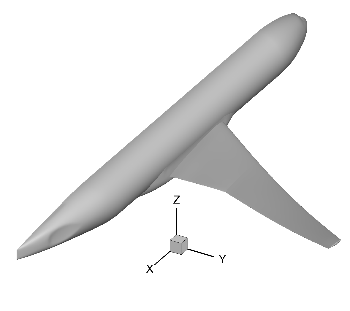
Fig. 7.2.3 Axis conventions demonstrated using the CRM geometry#

Table 7.2.4 Force and Moment output conventions.#

File

Output

total_forces_v2.csv, surface_forces_v2.csv and WebUI

\(CFx, CFy, CFz\)

Force coefficients (global axes)

-||-

\(CMx, CMy, CMz\)

Moment coefficients (global axes)

-||-

\(CL = CFz\cdot cos(\alpha) - CFx\cdot sin(\alpha)\)

Lift coefficient (wind axes)

-||-

\(CD = CFx\cdot cos(\alpha) cos(\beta) -\) \(CFz\cdot sin(\alpha) cos(\beta)\)

Drag coefficient (wind axes)

Not available (calculate from body forces)

\(CS = CFy\cdot cos(\beta) + CFx\cdot cos(\alpha) sin(\beta) -\) \(CFz\cdot sin(\alpha) sin(\beta)\)

Side force coefficient (wind axes)

total_forces_v2.csv, surface_forces_v2.csv

\(CFxPressure, CFyPressure, CFzPressure\)

Pressure contributions to force coefficients (global axes)

-||-

\(CMxPressure, CMyPressure, CMzPressure\)

Pressure contributions to moment coefficients (global axes)

-||-

\(CFxSkinFriction, CFySkinFriction,\) \(CFzSkinFriction\)

Skin friction contributions to force coefficients (global axes)

-||-

\(CMxSkinFriction, CMySkinFriction,\) \(CMzSkinFriction\)

Skin friction contributions to moment coefficients (global axes)

-||-

\(CLPressure, CDPressure\)

Pressure contributions to the lift and drag coefficients

-||-

\(CLSkinFriction, CDSkinFriction\)

Skin friction contributions to the lift and drag coefficients

bet_forces_v2.csv

\(Disk0\_Force\_x, Disk0\_Force\_y,\) \(Disk0\_Force\_z\)

BET Disk nondimensional forces (global axes)

-||-

\(Disk0\_Moment\_x, Disk0\_Monent\_y,\) \(Disk0\_Moment\_z\)

BET Disk nondimensional moments (global axes)

The BET disk forces and moments are calculated based on the global coordinate system (inertial reference frame). The BET disk moments are based on the center of rotation and rotor radius of each BET disk. The nondimensional factors used for the forces and moments are explained in more detail in the following sections.

7.2.3.1. CRM Wing-Body#

For the CRM wing body, the output coefficient values are averaged over the last 10% steps (500 iterations). The output coefficient values are shown in Table 7.2.5, with the pitching moment coefficient being equivalent to CMy in this case. The lift and pitching moment coefficients can be converted into dimensional units using the following equations:

(7.2.4)#\[\begin{split}L &= CL \cdot 0.5 \rho_\infty U_{ref}^2 A_{ref} = \\ &= CL \cdot 0.5 \rho_\infty \cdot M_\infty^2 C_\infty^2 \cdot \text{"geometry/refArea"} \cdot L_{gridUnit}^2 \\ M &= CM \cdot 0.5 \rho_\infty U_{ref}^2 A_{ref} L_{ref}= \\ &= CM \cdot 0.5 \rho_\infty \cdot M_\infty^2 C_\infty^2 \cdot \text{"geometry/refArea"} \cdot \text{"geometry/momentLength"} \cdot L_{gridUnit}^3\end{split}\]
Table 7.2.5 Lift and pitching moment coefficients from the CRM wing-body simulation#

Coefficient

Value

\(CL\)

0.6056

\(CM\)

-0.12462

An example of converting the lift and pitching moment coefficients (other forces and moments are equivalent) into dimensional units is shown in Table 7.2.6 for a number of different mesh units following the equations above.

Table 7.2.6 Conversion from coefficient values to dimensional forces for the CRM wing-body#

Units

Lift

Moment

Unit Chord

\(L = 0.6056 \cdot 0.5 \cdot 1.225 kg/m^3 \cdot 0.85^2 \cdot\) \(340.29^2 m^2/s^2 \cdot 3.909255 \cdot\) \(7.00532^2 m^2 =\) \(5953.579 kN\)

\(M = -0.12462 \cdot 0.5 \cdot 1.225 kg/m^3 \cdot 0.85^2 \cdot\)\(340.29^2 m^2/s^2 \cdot 3.909255 \cdot 1.0 \cdot\)\(7.00532^3 m^3 =\) \(-8,582.385 kN\cdot m\)

Inches

\(L = 0.6056\cdot0.5 \cdot 1.225 kg/m^3 \cdot 0.85^2 \cdot\) \(340.29^2 m^2/s^2 \cdot 297360 \cdot 0.0254^2 m^2 =\) \(5953.579 kN\)

\(M = -0.12462\cdot0.5 \cdot 1.225 kg/m^3 \cdot 0.85^2 \cdot\)\(340.29^2 m^2/s^2 \cdot 297360 \cdot 275.8 \cdot\)\(0.0254^3 m^3 =\) \(-8,582.385 kN\cdot m\)

Feet

\(L = 0.6056\cdot0.5 \cdot 1.225 kg/m^3 \cdot 0.85^2 \cdot\) \(340.29^2 m^2/s^2 \cdot 2065 \cdot 0.3048^2 m^2 =\) \(5953.579 kN\)

\(M = -0.12462\cdot0.5 \cdot 1.225 kg/m^3 \cdot 0.85^2 \cdot\)\(340.29^2 m^2/s^2 \cdot 2065 \cdot\)\(22.98333 \cdot\)\(0.3048^3 m^3 =\) \(-8,582.385 kN\cdot m\)

Metres

\(L = 0.6056\cdot0.5 \cdot 1.225 kg/m^3 \cdot 0.85^2 \cdot\) \(340.29^2 m^2/s^2 \cdot 191.844778 \cdot 1^2 m^2 =\) \(5953.579 kN\)

\(M = -0.12462\cdot0.5 \cdot 1.225 kg/m^3 \cdot 0.85^2 \cdot\)\(340.29^2 m^2/s^2 \cdot 191.844778 \cdot\)\(7.00532 \cdot 1^3 m^3 =\) \(-8,582.385 kN\cdot m\)

Millimetres

\(L = 0.6056\cdot0.5 \cdot 1.225 kg/m^3 \cdot 0.85^2 \cdot\) \(340.29^2 m^2/s^2 \cdot 191.844 \times 10^6 \cdot\)\(0.001^2 m^2 =\) \(5953.579 kN\)

\(M = -0.12462\cdot0.5 \cdot 1.225 kg/m^3 \cdot 0.85^2 \cdot\)\(340.29^2 m^2/s^2 \cdot 191.844 \times 10^6 \cdot\)\(7005.32\cdot 0.001^3 m^3 =\) \(-8,582.385 kN\cdot m\)

As can be seen from the example above, the coefficient values are independent of the mesh units used. When converting to dimensional forces, the product of the nondimensional reference area (geometry->refArea) and \(L_{gridUnit}^2\) is constant across different mesh units for the force conversion. For the moment conversion, the product of the nondimensional reference area (geometry->refArea), nondimensional reference length (geometry->momentLength) and \(L_{gridUnit}^3\) is fixed.

Note

When simulating a semi span airplane (like we have done above) the reference area must be properly set. If we want to get the forces on the whole aircraft from the semi span coefficients we should multiply the semi span refArea by 2.

7.2.3.2. Time-marching XV-15 Rotor Blade#

The example of the time-marching XV-15 rotor blade is not significantly different from the CRM wing-body case. In this case, the forces and moments are typically averaged over a revolution or number of revolutions (2 revolutions used here). As the rotor is in hover with the z-axis pointing upwards, the CFz value represents the thrust coefficient, whereas the CMz value represents the torque coefficient (note a 0.5 is used here in the denominator which is according to UK conventions). The resulting thrust and torque coefficients (CFz and CMz) are shown in Table 7.2.7. In this case, the rotor thrust and torque can be obtained using the following equations:

(7.2.5)#\[\begin{split}T &= CFz \cdot 0.5 \rho_\infty U_{ref}^2 A_{ref} =\\ &= CFz \cdot 0.5 \rho_\infty \cdot M_\infty^2 C_\infty^2 \cdot \text{"geometry/refArea"} \cdot L_{gridUnit}^2\\ Q &= CMz \cdot 0.5 \rho_\infty U_{ref}^2 A_{ref} L_{ref} =\\ &= CMz \cdot 0.5 \rho_\infty \cdot M_\infty^2 C_\infty^2 \cdot \text{"geometry/refArea"} \cdot \text{"geometry/momentLength"} \cdot L_{gridUnit}^3\end{split}\]
Table 7.2.7 Thrust and torque coefficients from the XV-15 rotor blade time-marching simulation#

Coefficient

Value

CFz

0.017001

CMz

0.001955

As mentioned previously, the primary difference between fixed-wing and rotor calculations, is the fact that for rotor calculations, the nondimensional reference area (geometry->refArea) is typically taken as the rotor disk area scaled by \(L_{gridUnit}^2\), whereas the rotor radius scaled by \(L_{gridUnit}\) is typically used as the nondimensional reference length (geometry->momentLength). Here, since the freestream velocity is zero then the Mach is also zero. We thus use the blade tip Mach number as the reference Mach number. An example of obtaining the dimensional thrust and torque values for a number of units is shown in Table 7.2.8. Similarly as for the CRM wing-body example, the coefficient values are independent of the mesh units used.

Table 7.2.8 Conversion from coefficient values to dimensional forces for the XV-15 rotor blade time-marching simulation#

Units

Thrust

Torque

Unit Chord

\(T= 0.017001 \cdot0.5 \cdot 1.225 kg/m^3 \cdot 0.69^2 \cdot\) \(340.29^2 m^2/s^2 \cdot 360.623 \cdot\) \(0.3556^2 m^2 =\) \(26179.06N\)

\(Q = 0.001955\cdot0.5 \cdot 1.225 kg/m^3 \cdot 0.69^2 \cdot\)\(340.29^2 m^2/s^2 \cdot 360.623 \cdot 10.714 \cdot\)\(0.3556^3 m^3 =\) \(11469.37 N\cdot m\)

Inches

\(T= 0.017001 \cdot0.5 \cdot 1.225 kg/m^3 \cdot 0.69^2 \cdot\) \(340.29^2 m^2/s^2 \cdot 70,685.835 \cdot\) \(0.0254^2 m^2 =\) \(26179.06N\)

\(Q = 0.001955\cdot0.5 \cdot 1.225 kg/m^3 \cdot 0.69^2 \cdot\)\(340.29^2 m^2/s^2 \cdot 70,685.834 \cdot 150 \cdot\)\(0.0254^3 m^3 =\) \(11469.37 N\cdot m\)

Feet

\(T= 0.017001 \cdot0.5 \cdot 1.225 kg/m^3 \cdot 0.69^2 \cdot\) \(340.29^2 m^2/s^2 \cdot 490.874 \cdot\) \(0.3048^2 m^2 =\) \(26179.06N\)

\(Q = 0.001955\cdot0.5 \cdot 1.225 kg/m^3 \cdot 0.69^2 \cdot\)\(340.29^2 m^2/s^2 \cdot 490.874 \cdot 12.5 \cdot\) \(0.3048^3 m^3 =\) \(11469.37 N\cdot m\)

Metres

\(T= 0.017001 \cdot0.5 \cdot 1.225 kg/m^3 \cdot 0.69^2 \cdot\) \(340.29^2 m^2/s^2 \cdot 45.6037 \cdot 1^2 m^2 =\) \(26179.06N\)

\(Q = 0.001955\cdot0.5 \cdot 1.225 kg/m^3 \cdot 0.69^2 \cdot\)\(340.29^2 m^2/s^2 \cdot 45.6037 \cdot 3.81 \cdot 1^3 m^3 =\) \(11469.37 N\cdot m\)

Millimetres

\(T= 0.017001 \cdot0.5 \cdot 1.225 kg/m^3 \cdot 0.69^2 \cdot\) \(340.29^2 m^2/s^2 \cdot 45.6037 \times 10^6 \cdot\) \(0.001^2 m^2 =\) \(26179.06N\)

\(Q = 0.001955\cdot0.5 \cdot 1.225 kg/m^3 \cdot 0.69^2 \cdot\)\(340.29^2 m^2/s^2 \cdot 45.6037 \times 10^6 \cdot 3810 \cdot\) \(0.001^3 m^3 =\) \(11469.37 N\cdot m\)

7.2.3.3. BET Disk XV-15 Rotor Blade#

The conversion of the forces and moments from the BET Disks is slightly different as the values are independent of the reference area and length specified in the Flow360.json file. This means that the nondimensional force and moment outputs in bet_forces_v2.csv vary depending on the mesh unit used. The dimensional thrust and torque values can be obtained using the following equations (assuming the rotor disk is aligned with z-axis pointing upwards):

(7.2.6)#\[\begin{split}T = Disk\_Force\_z \cdot \rho_\infty C_\infty^2 L_{gridUnit}^2\\ Q = Disk\_Moment\_z \cdot \rho_\infty C_\infty^2 L_{gridUnit}^3\end{split}\]

The values obtained from the BET simulation using different mesh units for the Disk nondimensional z-force and moment about the z-axis are shown in Table 7.2.9

Table 7.2.9 nondimensional thrust and torque from the XV-15 rotor blade BET disk simulation.#

Unit

Disk_Force_z

Disk_Moment_z

Unit Chords

1.4073

1.1510

Inches

275.8400

3158.2089

Feet

1.9156

1.8277

Metres

0.1780

0.0518

Millimetres

177960.9339

51753770.9889

In this case, the nondimensional thrust and torque values vary with the mesh units used, however, all simulations lead to the same dimensional forces and moments. An example of obtaining the dimensional thrust and torque values for a number of units is shown in Table 7.2.10.

Table 7.2.10 Conversion from coefficient values to dimensional forces for the XV-15 rotor blade BET disk simulation#

Units

Thrust

Torque

Unit Chord

\(T= 1.4073 \cdot 1.225 kg/m^3 \cdot\) \(340.29^2 m^2/s^2 \cdot 0.3556^2 m^2 =\) \(25244.056N\)

\(Q = 1.1510 \cdot 1.225 kg/m^3 \cdot\)\(340.29^2 m^2/s^2 \cdot 0.3556^3 m^3 =\) \(7341.359 N\cdot m\)

Inches

\(T= 275.840 \cdot 1.225 kg/m^3 \cdot\) \(340.29^2 m^2/s^2 \cdot 0.0254^2 m^2 =\) \(25244.056N\)

\(Q = 3158.2089 \cdot 1.225 kg/m^3 \cdot\)\(340.29^2 m^2/s^2 \cdot 0.0254^3 m^3 =\) \(7341.359 N\cdot m\)

Feet

\(T= 1.9156 \cdot 1.225 kg/m^3 \cdot\) \(340.29^2 m^2/s^2 \cdot 0.3048^2 m^2 =\) \(25244.056N\)

\(Q = 1.8277 \cdot 1.225 kg/m^3 \cdot\)\(340.29^2 m^2/s^2 \cdot 0.3048^3 m^3 =\) \(7341.359 N\cdot m\)

Metres

\(T= 0.1780 \cdot 1.225 kg/m^3 \cdot\) \(340.29^2 m^2/s^2 \cdot 1^2 m^2 =\) \(25244.056N\)

\(Q = 0.0518 \cdot 1.225 kg/m^3 \cdot\)\(340.29^2 m^2/s^2 \cdot 1^3 m^3 =\) \(7341.359 N\cdot m\)

Millimetres

\(T= 177960.9339 \cdot 1.225 kg/m^3 \cdot\) \(340.29^2 m^2/s^2 \cdot 0.001^2 m^2 =\) \(25244.056N\)

\(Q = 51753770.9889 \cdot 1.225 kg/m^3 \cdot\)\(340.29^2 m^2/s^2 \cdot 0.001^3 m^3 =\) \(7341.359 N\cdot m\)

This completes the tutorial on nondimensionalization conventions in Flow360. A short note on the results can be made, comparing results between the XV-15 time-marching and BET disk simulations. The dimensional thrust shows good agreement, however, the BET disk simulation predicts a much lower torque than the time-marching simulation. This is primarily due to the fact that very coarse grids were used in these simulations, hence the boundary layer is not well resolved for the time-marching simulation. The main purpose of this tutorial was to demonstrate the different nondimensionalization conventions used in Flow360.