6.1. Geometry Modeling and Preparation for Automated Meshing: An Example of the ONERA M6 Wing#
In this tutorial, we explain how to build the ONERA M6 Wing Model in Engineering Sketch Pad (ESP) and how to use edge, face, and group attributes to prepare the model for automatic meshing. More information about ESP installation is available here. To build the geometry through ESP, we use a series of statements and commands in a scripted fashion. This gives us the ability to rebuild and modify the model most efficiently. All ESP statements and commands are held in a *.csm file. ESP uses the OpenCSM (Open-source Constructive Solid Modeling) system which is a feature-based, associative, parametric solid modeler. The input to OpenCSM is an ASCII, human-readable *.csm file that is used to describe the model through a series of design parameters and a build prescription. In this tutorial, users are expected to be comfortable with parametric modeling and scripting via ESP.
The ONERA M6 Wing Model is based on the geometric layout on Page 38 of the Schmitt and Charpin report. More details about this geometry are provided in this link.
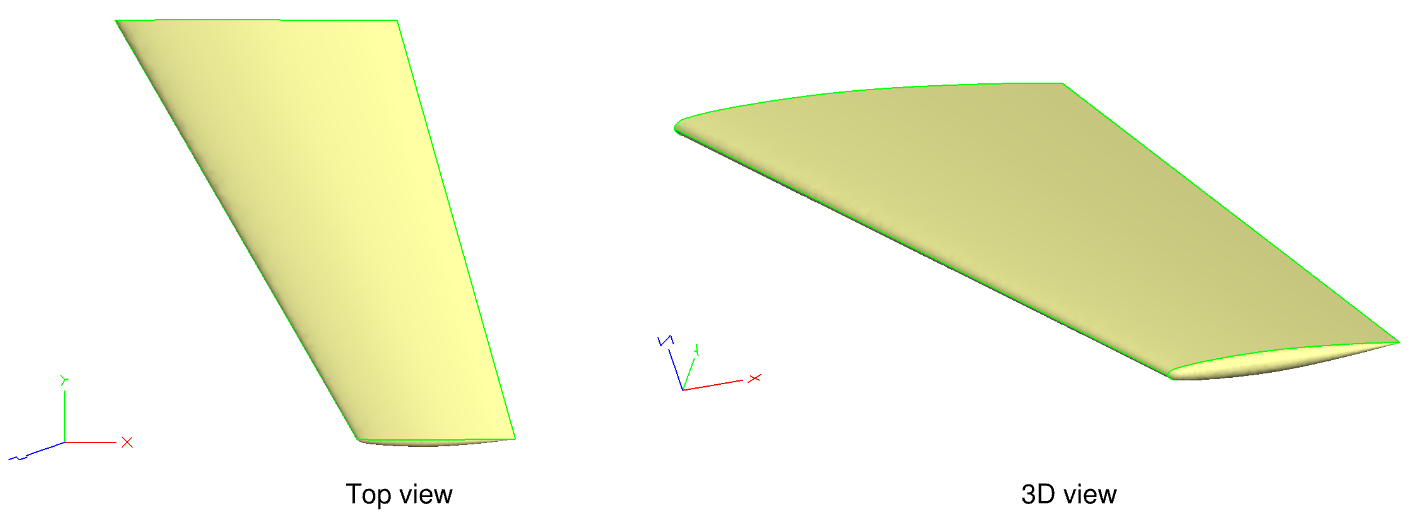
Fig. 6.1.1 ONERA M6 Wing generated in ESP#
Details of the ONERA M6 Wing geometry in this tutorial are:
Root chord: 0.8059 m
Leading-edge Sweep: 30.0 °
Trailing-edge Sweep: 15.8 °
Semi-span: 1.1963 m
Taper ratio: 0.56
Rounded Tip Semi-span: 1.219526 m
Note
There is another CAD geometry for the ONERA M6 Wing with slightly different specifications in the NASA Turbulence Modeling Resource website. In that CAD model, referenced in this paper, 0.55 percent is added to the local chord to add a sharp trailing edge. The paper concludes that the effect of a sharp trailing edge on the Cp distribution is very small.
3D Sketches of Airfoils#
The first step to building the wing is to create 3D sketches for the root and tip airfoils. We will use the following CSM statements to create 3D airfoil sketches.
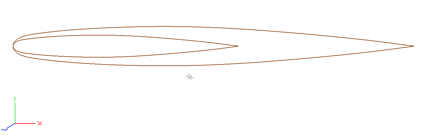
Fig. 6.1.2 3D Sketches of Root and Tip Airfoils#
MARK use: used to identify groups such as in RULE, BLEND, or GROUP
The CSM statement mark is used to identify groups of entities. In this example, we use mark to identify a sketch group for the root and another sketch group for the tip.
SKBEG x y z relative=0 use: start a new Sketch with the given point
The skbeg statement is used to start a sketch. The following x, y, z define the starting point for the sketch. The fourth argument indicates whether values inside the sketch are relative to the starting point or not.
Inside the sketch, we define a spline point by point. Every point is considered a control point for the spline. The spline statement is described below:
SPLINE x y z use: add a point to a spline
We finish the sketch by using skend.
SKEND wireonly=0 use: completes a Sketch
For each root and tip airfoils, we separately define the upper and lower curves. Then, we group them in order to later translate them. We also store them after putting them into a group to be able to retrieve them from the stack. The group and store commands are as follows:
GROUP nbody=0 use: create a Group of Bodys since Mark for subsequent transformations
STORE $name index=0 keep=0 use: stores Group on top of Stack
At this stage the CSM file looks like this:
mark
skbeg   up_x_TE  up_y_TE  up_z_TE
spline  up_x_p1  up_y_p1  up_z_p1
.
.
.
spline  up_x_LE  up_y_LE  up_z_LE
skend

skbeg   low_x_LE  low_y_LE  low_z_LE
spline  low_x_p1  low_y_p1  low_z_p1
.
.
.
spline  low_x_TE  low_y_TE  low_z_TE
skend
group
store airfoil
The above CSM example shows how to put together a 3D sketch for an airfoil. These 3D sketches are later used to build a face body and then face bodies are used to be blended into a solid body. For that reason, the face orientation, and number of edges in a face must be consistence in all cross sections. The face orientation depends on the direction of the control points defining a spline. In that case, all 3D sketches start from the upper trailing-edge point to the leading-edge point and back to the lower trailing-edge point. This means the points definition is counter-clockwise. If you happen to be familiar with XFOIL, you will note that the 2D section point definitions are defined in the same order.
Here you can find the complete CSM file for step one: om6Step1.csm.
ESP has different coloring schemes, which can be selected by clicking on DisplayType. The default coloring scheme is 0 monochrome in which:
Faces associated with SolidBodys are light yellow
Faces associated with SheetBodys are light red
Edges that were created as part of a primitive operation are green
Edges that were created by a Boolean or Applied Branch are blue
Edges that have only one associated Face are brown
Edges that have more than two associated Faces are orange
Nodes are small black squares
Wing Planform#
In this step, we define the wing planform based on the geometric layout referenced above, then we elevate sketches to faces and translate them.
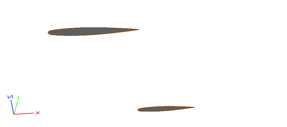
Fig. 6.1.3 Wing Planform With of Root and Tip Faces#
To create the planform, we define two parameters: span and leading-edge sweep angle. We assume that ‘span’ here, is a design parameter and later we might want to change it and ‘leading-edge sweep’ is a constant parameter in our configuration. To do that we use the following two CSM statements.
DESPMTR $pmtrName values use: define a design Parameter
CONPMTR $pmtrName values use: define a constant Parameter
Then, we restore a sketch group that represents an airfoil and join the sketch bodies for the upper and lower splines into a single sketch body. This sketch group could be the tip airfoil or the root airfoil for the ONERA M6 Wing. These sketch groups are stored earlier in the build process.
RESTORE $name index=0 use: restores Body(s) that was/were previously stored
JOIN toler=0 toMark=0 use: join two Bodys at a common Edge or Face
Since the aforementioned sketches are in the xy-plane, we need to rotate them around the x-axis in order to align the span with the y-axis.
ROTATEX angDeg yaxis=0 zaxis=0 use: rotates Group on top of Stack around an axis that passes through (0, yaxis, zaxis) and is parallel to the x-axis
We use translate to move the tip sketch group to the correct position in space. The leading edge line for the wing root sketch starts at the origin 0,0,0. Then, span/tand(90-LEsweep) is the x-coordinate of the tip face leading edge. Since we model the wing along the negative y-axis, -span is the spanwise coordinate.
TRANSLATE dx dy dz use: translates Group on top of Stack
After the the sketch body is moved, we use combine to elevate the sketch body into a face.
COMBINE toler=0 use: combine Bodys since Mark into next higher type
At the end, we store the face to be able to restore it later. Here you can find the complete CSM file for step two: om6Step2.csm.
Wing Solid Model#
In this step we create the wing solid body by using blend.
BLEND begList=0 endList=0 reorder=0 oneFace=0 periodic=0 use: create a Body by blending through Xsects since Mark
The rounded tip is created by using an endList in front of the BLEND. This endList = “-1;1.1” indicates that the rounded end has an aspect ratio of 1.1.
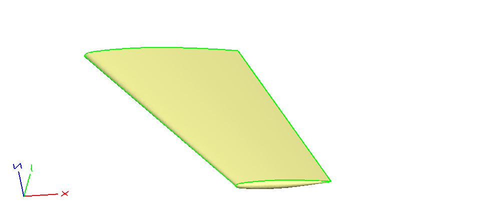
Fig. 6.1.4 OM6 Wing Solid Body With Rounded Wingtip#
Here you can find the CSM file for step three: om6Step3.csm.
In the Graphic window, bodies are included in the Display part of the tree window to the left. The listing can be expanded by pressing + to the left and Faces, Edges, and Nodes can be seen. To the right of each, you will find the items below:
Viz: toggles the visibility
Grd: toggles the internal tessellation grid
Trn: toggles the pseudo-transparency
Ori: toggles the orientation
Alternatively, when you hover over an entity, you can press:
v to toggle the visibility
g to toggle the grid
t to toggle the transparency
o to toggle the orientation
Adding Edge Attribute#
We use edge attributes to have control over the unstructured surface mesh. We assign attributes to edges and groups of edges so that we can then later assign surface meshing parameters to each edge or group of edges. These attributes, when combined with an appropriate surface mesh JSON file, indicate the types and values of meshing parameters. There are different approaches to assigning attributes to edges. We will show you three methods below.
The first method allows you to generically add the edge attributes in your model within the build prescription, maintain the attributes and be able to change the design parameters. However, it could be challenging for a build process to obtain identity numbers of the edges based on the geometric features. The second method uses a bounding box to select edges and assign attributes. The challenge in this method is that the bounding box could encompass other edges with different edge attributes. In addition, defining the input values of the bounding box could be challenging beforehand. The third method uses edge IDs to select edges and assign attributes. The challenge in this method is that we cannot know the edge IDs before completing the build process. In addition, since the ID number could change for each build process, using ID numbers specifically to select edges is not recommended.
Depending on the model complexity and intended geometry variations, one or more of these techniques can be used to add attributes to the edges for the purposes of automatic meshing. Scripting the edge attributes for inclusion in the build prescription, as described in the first method, allows you to have a generic build process for geometry variation and assessment. The second method allows you to select a group of edges at once, add an edge attribute to all of them, and skip the complexity of identifying associated nodes. The third method allows you to postprocess a build prescription and quickly add the edge attributes based on the associated edge ID from the build tree without going into details of the build process.
Using Coordinates of Nodes and Edge Attribute UDPRIM#
In this method, for a solid body, we collect and store the identity of all the nodes. All nodes are identifed by a number. Then we use UDPRIM edgeAttr to add a name to an edge by using the coordinates of edge nodes. The challenge is to be able to identify different nodes in different parts of a solid body. We assume we are not aware of node IDs beforehand and node IDs could change when the solid body is built on different systems or architectures. In addition, we would like to have the ability to change the design parameters during the build process and still be able to add the same attributes to the same edges.
In order to do that, we need to know how many nodes are in a solid body. Then we loop over all the nodes and store their IDs based on their location in the topology. Later, we use that stored ID to differentiate nodes and use their coordinates to add an edge attribute.
For example, an airfoil on xz-plane with x-axis along the chordwise direction, will have minimum x at the leading-edge, which defines the leading-edge node ID. The other two node IDs will form the upper trailing-edge node with maximum z and the lower trailing-edge node with minimum z. In this way we can find leading-edge, upper and lower trailing-edge nodes.
Note
In this tutorial, a “bottom up” approach is provided to construct the wing. The solid body is built up from nodes, to curves, to edges, to surfaces, to faces, to shells, and finally bodies. The term ‘node’ here refers to the nodes at the ends of each edge, which differs from the airfoil data points used to define the upper and lower curves.
For example, for an airfoil with three nodes at the leading-edge and the upper/lower trailing-edge, we can sort the nodes like this:
# defining arrays with one row and three columns
dimension rootLeadingPoint  1 3
dimension rootTrailingPointUp 1 3
dimension rootTrailingPointLow 1 3

# initializing xmin, zmin, zmax with their opposite extremes
set xmin @xmax
set zmin @zmax
set zmax @zmin

# looping over nodes to find the LE
set numNodes @nnode
patbeg inode numNodes
    evaluate node @ibody inode
    IFTHEN @edata[1] LT xmin
        set xmin @edata[1]
        set rootLeadingPoint "xmin;@edata[2];@edata[3];"
        set leadingNodeID inode
    ENDIF
patend

# looping over nodes to find the TE
patbeg inode numNodes
    IFTHEN inode NE leadingNodeID
        evaluate node @ibody inode
        IFTHEN @edata[3] GT zmax
            set zmax @edata[3]
            set rootTrailingPointUp  "@edata[1];@edata[2];zmax;"
        ENDIF

        IFTHEN @edata[3] LT zmin
            set zmin @edata[3]
            set rootTrailingPointLow "@edata[1];@edata[2];zmin;"
        ENDIF
    ENDIF
patend
In the above code, dimension declares the array and its size.
DIMENSION $pmtrName nrow ncol use: set up or redimensions an array Parameter
Next, we initialize xmin, zmin, and zmax with their polar extremes. For clarity, the lines of the code doing the initialization are highlighted.
The statement @nnode gives us the number of nodes in the current body. @xmax, @zmax, and @zmin give us the maximum and minimum values of x and z of the bounding box for the current body. The current body can be accessed by @ibody. In order to obtain the node coordinates, we use evaluate.
EVALUATE $type arg1 … use: evaluate coordinates of NODE, EDGE, or FACE
After the evaluate statement, evaluated data can be accessed by using the **edata** array.
For example, after:
evaluate node @ibody 1
The edata[1], [2], [3] variables contain the x, y, and z coordinates of the current body at nodeId = 1. In order to loop over nodes, we use patbeg and patend.
PATBEG $pmtrName ncopy use: execute a Block of Branches ncopy times
And we use IFTHEN and ENDIF to define a conditional statement in our CSM script.
IFTHEN val1 $op1 val2 $op2=and val3=0 $op3=eq val4=0 use: execute or skip a Block of Branches
In the above code, at each loop, after we evaluate a node in a solid body, if the x-coordinate has a value less than the current value of xmin, we update the xmin value with a new value and store the ID of that node. In this way, by looping over all the nodes and starting from maximum x as initial value of xmin, we find the node ID that has the minimum x. We store the x,y,z coordinates of that node as the leading-edge coordinates. This conditional statement is also highlighted in the example.
We repeat the same process for the rest of nodes to find the node with the maximum z value and the node with the minimum z value. In the above example, these two conditional statements are also highlighted. We store the x,y,z coordinates of these nodes as upper trailing-edge and lower trailing-edge respectively. Again, in order to find them, we initialize the zmax and zmin with their polar extremes, and update their values at each loop. With this technique, we need to collect coordinates of the nodes when we build the faces. Since each face is a solid body, we use evaluate at all the nodes of a face to find the nodes with the maximum and minimum values. After we have stored the coordinates of the leading-edge and trailing-edge nodes in their arrays, we use the UDPRIM edgeAttr command to add an attribute to each edge using its coordinates.
udparg edgeAttr attrname $edgeName  attrstr $wingLeadingEdge
udprim edgeAttr xyzs "rootLeadingPoint[1];rootLeadingPoint[2];rootLeadingPoint[3];tipLeadingPoint[1];tipLeadingPoint[2];tipLeadingPoint[3];"

udparg edgeAttr attrname $edgeName  attrstr $wingTrailingEdge
udprim edgeAttr xyzs "rootTrailingPointUp[1];rootTrailingPointUp[2];rootTrailingPointUp[3];tipTrailingPointUp[1];tipTrailingPointUp[2];tipTrailingPointUp[3];"

udparg edgeAttr attrname $edgeName  attrstr $wingTrailingEdge
udprim edgeAttr xyzs "rootTrailingPointLow[1];rootTrailingPointLow[2];rootTrailingPointLow[3];tipTrailingPointLow[1];tipTrailingPointLow[2];tipTrailingPointLow[3];"
In the above code, udparg edgeAttr attrname $edgeName attrstr is followed by a string starting with ‘$’. This string is the input argument to the UDPRIM edgeAttr. Then, udprim edgeAttr xyzs is followed by the coordinates of starting and ending nodes of the edge enclosed in double quotes.
Later, we use the keyword string assigned here, and also in the surface mesh JSON file to assign the type and value of meshing parameters to this edge. In each array, indices 1, 2 and 3 indicate x, y, and z.
The challenge with this method is to sort the nodes based on the specific topology of the design. Things like, for example, the maximum and minimum values of x, or any other particular feature in a solid body that can be used to programmatically differentiate nodes.
Here you can find the complete CSM file for step four, method one: om6Step4Method1.csm. You can see the results in Fig. 6.1.5, by running the above CSM file in ESP using the command:
serveCSM om6Step4Method1.csm
You can see the edgename attribute in the message panel by holding the mouse over the edge and pressing 6.
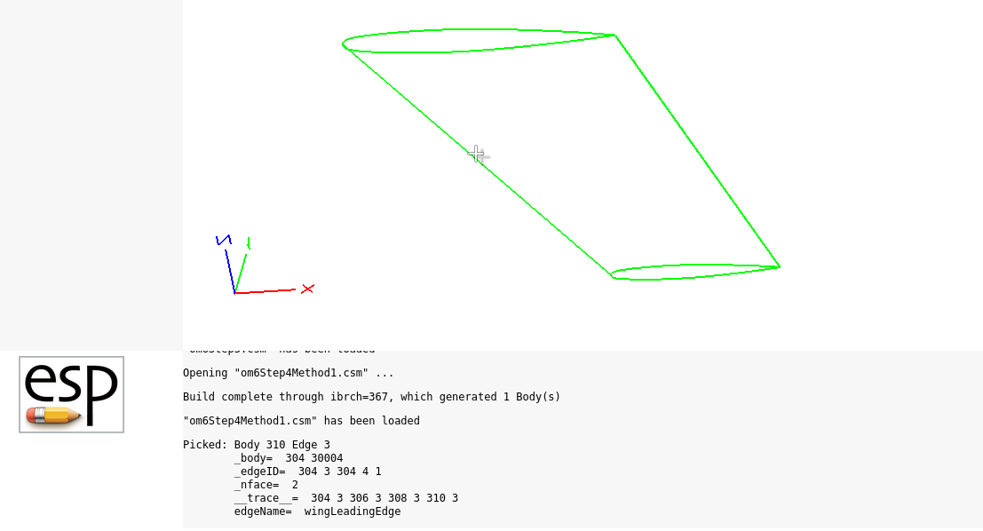
Fig. 6.1.5 OM6 Wing Edge Attribute on Leading-edge#
Using a Bounding Box#
In this method, we define a bounding box using extrema in three directions. Then, we select all the edges in that bounding box and add attributes to them.
select edge @xmin @xmax -0.01 0.01 @zmin @zmax
attribute edgeName $rootAirfoilEdge
The definition and usage of select can be found below:
SELECT $type arg1 … use: selects entity for which @-parameters are evaluated
In the above code, we defined a bounding box with @xmin and @xmax corresponding to the minimum and maximum x values, -0.01 and 0.01 corressponding to minimum and maximum y values, and @zmin and @zmax corresponding to minimum and maximum z values. This line is highlighted. All edges in this bounding box will be have an attribute edgeName of rootAirfoilEdge.
Here you can find the CSM file for step four, method two: om6Step4Method2.csm. As shown in Fig. 6.1.6, after launching the above CSM file in ESP by running:
serveCSM om6Step4Method2.csm
You can see the edgename attribute in the message panel by pressing 6 over the edge.
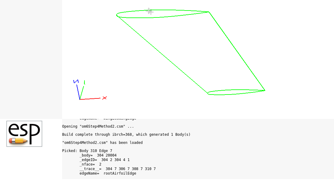
Fig. 6.1.6 OM6 Wing Edge Attribute on Root Edge#
Using Edge ID#
In this method, we assume the edge ID for a particular edge is already known. We select the edge using its ID and add the attribute to the edge.
select edge 2
attribute edgeName $tipAirfoilEdge

select edge 5
attribute edgeName $tipAirfoilEdge
In the above statements, 2 and 5 are IDs for edges at the wingtip. The challenge in this method is that we do not always know the ID number for edges, and in general, it is not recommended to use the ID to select an edge, face or body because there is no guarantee that the ID remains the same in a different build process, on different computers or with different ESP versions. This general recommendation comes from the ESP help documentation.
Here you can find the complete CSM file for method 3: om6Step4Method3.csm.
You can launch the CSM file by running this command in your terminal within ESP:
serveCSM om6Step4Method3.csm
As shown in the Fig. 6.1.7, in order to check whether the edge attributes are added correctly, you can build the model, turn off Viz for faces, and while holding the mouse over a particular edge, press 6 to check the attribute in the message panel.

Fig. 6.1.7 OM6 Wing Edge Attribute on Tip Edge#
Adding Face and Group Attributes#
After we have added edge attributes for a body, we need to add face attributes. The face attribute is used to have control over the resolution of the unstructured mesh at the time of preprocessing. The group attribute is used to lump together various faces into the relevant groups so that we can easily postprocess not only the whole object we have simulated but also analyze its subcomponents.
Since we want to add a face attribute to the whole solid body, we store the body at the end and then restore it. Then, we assign the face attribute. In this way, all faces in that body will have the same face attribute. Then, we add a group attribute to the whole solid body.
Since we want to add a face attribute to the whole solid body, we:
store the body at the end of its creation stage
restore the body to make it the current body
assign the face attribute
In this way, all the faces in that body will have the same face attribute.
store wingModel

restore wingModel
attribute faceName $wing
attribute groupName $wing
After adding the face and group attribute, which is shown in the above example, since we want to have the same grid settings to compare with the NASA Turbulence Modeling Resource website , we set root chord = 1 by scaling the whole solid body with 1/0.8059 around the origin.
scale 1/0.8059 0 0 0
More information about the scale statement can be found below:
SCALE fact xcent=0 ycent=0 zcent=0 use: scales Group on top of Stack around given point
Here you can find the complete CSM file for step five: om6Step5.csm. The ONERA M6 Wing model in ESP is shown in Fig. 6.1.8. You can launch the CSM file by running this command in your terminal:
serveCSM om6Step5.csm
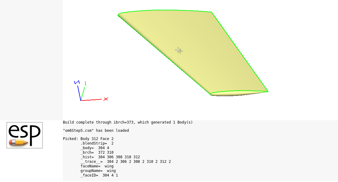
Fig. 6.1.8 OM6 Wing Face and Group Attributes#