6.10. DTU 10MW Wind Turbine

6.10.1. Introduction

The purpose of this case study is to validate and demonstrate the application of Flow360 to wind turbine simulations. A common research wind turbine model, the DTU 10MW Reference Wind Turbine (RWT), was selected and unsteady compressible DDES simulations performed with the Spalart-Allmaras (SA) turbulence model. Flow conditions were simulated at the rated wind speed of 11m/s, which relate to the rated power output of 10MW. Off-design conditions with different wind speeds were also simulated.

6.10.2. Rotor Geometry

The wind turbine blade geometry was reproduced programmatically using 200 spanwise cross-sections along the blade and airfoil profiles extracted from the original source geometry (see Fig. 6.10.1). The fine resolution blade geometry from the GitLab repository of DTU 10MW RWT was used.

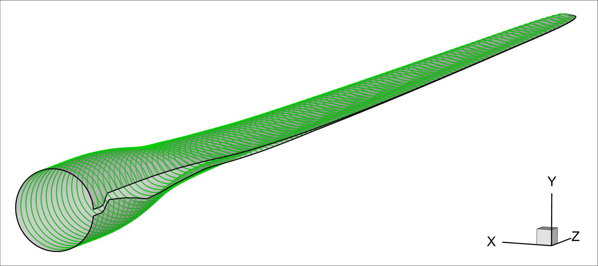
Fig. 6.10.1 Schematic of sectional airfoil profiles extracted. For clarity, only 100 cross-sections are shown.

The original blade geometry used is rigid with no aeroelastic deformations. Slight modifications were made at the blade tip to help improve unstructured mesh quality. Moreover, an elliptic fairing was added to reduce the downstream separation region around the blade roots. Fig. 6.10.2 displays an overlay of the geometry created here and the original. The current CAD model is an EGADS format and is available here.

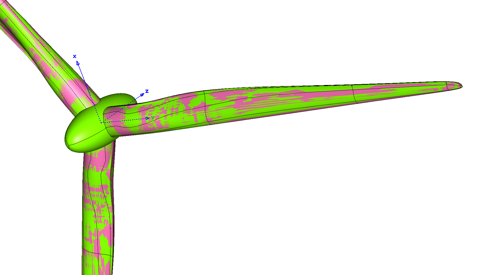
Fig. 6.10.2 Geometric comparison of wind turbine models (Red: original design, Green: current model).

6.10.3. Automated Meshing

A series of computational grids, with consecutively refined mesh resolution, were created with our automated meshing process. The corresponding key meshing parameters are summarized in Table 6.10.1. The volume mesh was consistently refined by a factor of \(2\). Additionally, the edge lengths orthogonal to curves, such as the leading edge (LE), the trailing edge (TE) and the blade tip, were refined by a factor of \(2^{1/3}\). A refinement factor of \(2^{2/3}\) was also applied to the max cell edge length on the blade and the tip faces. Notably, the target 1st layer thicknesses were kept as 1E-06 meters, but are influenced by the volumetric refinement factor. The 1st layer thickness values applied were meant to ensure \(y^+ < 1\) in all the cases. The farfield was automatically set to be about 7700 meters away from the rotor center.

Table 6.10.1 Mesh statistics

Parameters	Units	Coarse	Medium	Fine
Volume Mesh
Refinement Factor	—	1/2	1	2
1st Layer Thickness	m	1E-06	1E-06	1E-06
Growth Rate	—	1.2	1.2	1.2
Surface Mesh
Edge Length (LE)	deg	0.126	0.100	0.079
Edge Length (TE)	m	0.004	0.003	0.002
Edge Length (Tip)	m	0.063	0.050	0.040
Max Cell Edge Length (Blade)	m	0.317	0.200	0.126
Max Cell Edge Length (Tip)	m	0.159	0.100	0.063
Growth Rate	—	1.2	1.2	1.2
Mesh Statistics
Total Nodes	million	22	35	65
Total Cells	million	59	93	173

The medium mesh resolution is visualized in Fig. 6.10.3. The upper two frames display the rotor nearfield and a zoomed-in view, respectively. As seen in the upper left figure, a rotating mesh region surrounding the rotor was used with sliding interfaces and a maximum element edge length of 1 meter applied. To better resolve the downstream progression of tip vortices, an additional volumetric refinement region was introduced with a 2 meter cell spacing. The front and rear views of the surface mesh are shown in the lower left and lower right frames, respectively. Refinement of the surface mesh can be seen along the LE and TE, as well as at the blade root and tip.

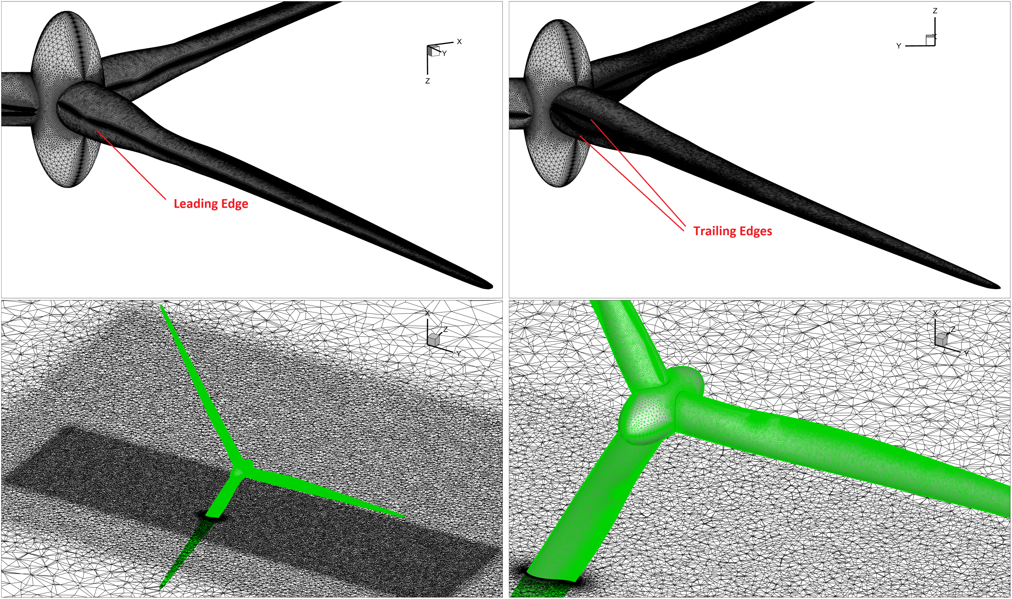
Fig. 6.10.3 Overview of surface and volume mesh (medium resolution).

The configuration json files are available through these links for the aforementioned surface (Coarse, Medium and Fine) and volume (Coarse, Medium and Fine) meshes, respectively.

6.10.4. Flow Configuration

The wind turbine operation was first simulated at the rated power condition, utilizing the three computational grids discussed above. Key flow configuration parameters are summarized in Table 6.10.2. Importantly, to extract power from the air, the rotor is designed for incoming wind to impinge on the pressure side of the turbine blades, so that the circumferential component of the aerodynamic lift drives the turbine rotation in the positive z-direction (right-hand rule). This is equivalent to setting the angle of attack, \(\alpha = +90\) °, in accordance with Flow360’s conventions. Additional details for solver settings are given in the Navier-Stokes and turbulence model knowledge bases.

Table 6.10.2 Key flow configuration parameters

Parameters	Units	Values	Notes
Geometry
\(L_{gridUnit}\)	\(m\)	1
\(A_{ref}\)	\(m^2\)	24977.47	\(\pi R_{tip}^2\)
\(L_{ref}\)	\(m\)	89.166	\(R_{tip}\)
Free Stream
\(T_{\infty}\)	\(K\)	288.15
\(\rho_{\infty}\)	\(kg/m^3\)	1.225
\(M_{\infty}\)	—	0.032325	\(U_{\infty}=11 m/s\)
\(M_{ref}\)	—	0.242454	\(U_{ref}=\omega R_{tip}\)
\(N\)	rpm	8.836	rotating speed
\(\alpha\)	deg	+90
\(\beta\)	deg	0

Unsteady DDES simulations were carried out through three consecutive stages. To initialize the flow field, the turbine operation was started with a physical time step size equivalent to rotating through \(6\) ° for three revolutions, utilizing 1st-order spatial schemes for both Navier-Stokes and turbulence model equations. This was followed by twelve revolutions with 2nd-order schemes through the second stage to further develop the flow. Finally, for time-accurate solutions, the physical time step size was reduced to \(3\) °, \(2\) ° and \(1\) ° per time step, according to the three grid levels, and simulations were carried on for another three revolutions. The solver configuration json files are available here (Stage-1, Stage-2, and Stage-3 with 3DegPerStep, 2DegPerStep and 1DegPerStep). More details about time integration settings are given in the time stepping knowledge base. The corresponding temporal evolutions of CFL numbers, nonlinear residuals, force and moment coefficients are shown in the next section for the case with the medium grid.

6.10.5. Residual Convergence

Within each physical time step, the CFL number is ramped up from 10 to 200 in 10 pseudo steps. The maximum number of pseudo steps within each physical time step is conservatively set to 100 to allow all nonlinear residuals to decrease by at least two orders of magnitude. Convergence of nonlinear residuals is shown in Fig. 6.10.4. For clarity, only continuity is displayed.

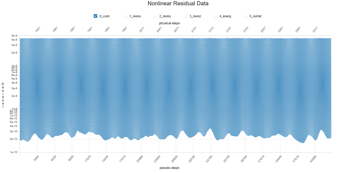
Fig. 6.10.4 Convergence of continuity nonlinear residual, medium grid, stage 3.

The temporal evolutions of force and moment coefficients are shown in Fig. 6.10.5 and Fig. 6.10.6. As seen, the aerodynamic loads seemed to be stabilized, with minor blade passing oscillations.

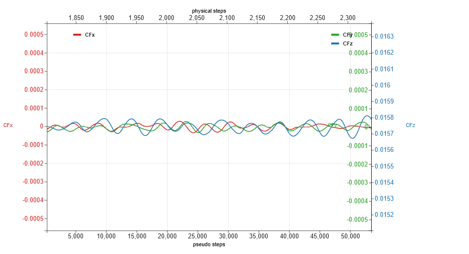
Fig. 6.10.5 Evolutions of force coefficients (CFx, CFy and CFz), medium grid, stage 3.

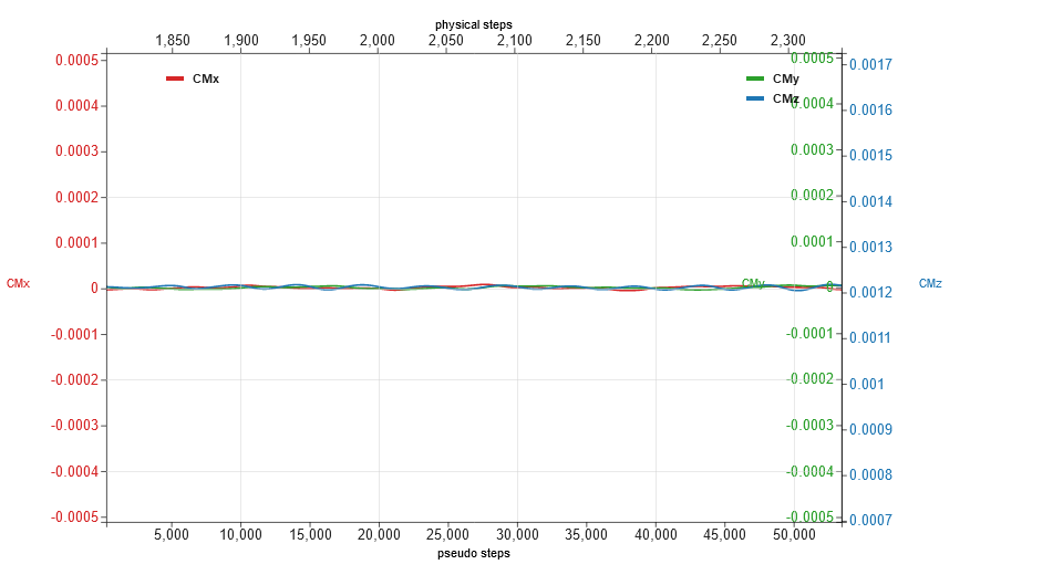
Fig. 6.10.6 Evolutions of moment coefficients (CMx, CMy and CMz), medium grid, stage 3.

6.10.6. Surface and Volumetric Results

Numerical results computed on the mesh of the medium resolution are examined in this section. Surface distributions of \(y^{+}\), \(C_{p}\) and \(C_{f}\), are displayed on one of the three blades, respectively. The elliptic fairing is contoured by \(C_{p}\). As seen, all values of \(y^{+}\) were less than \(1\). Also, as expected, the major fraction of power output was generated from the outer part of the span primarily by the pressure differences between the pressure and the suction sides.

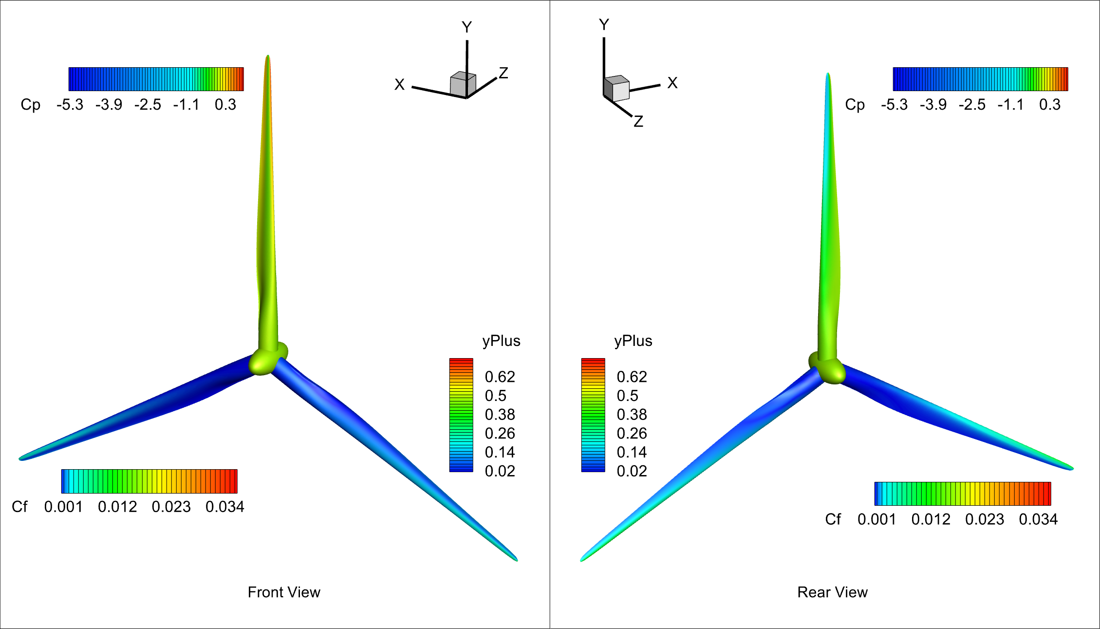
Fig. 6.10.7 Surface contours of \(y^{+}\), \(C_{p}\) and \(C_{f}\).

Tip vortices were identified by Q-criterion and visualized as shown in the next figure, which were contoured by Mach number. Root vortices separating off the fairing, as well as the Gurney flaps, were also identified.

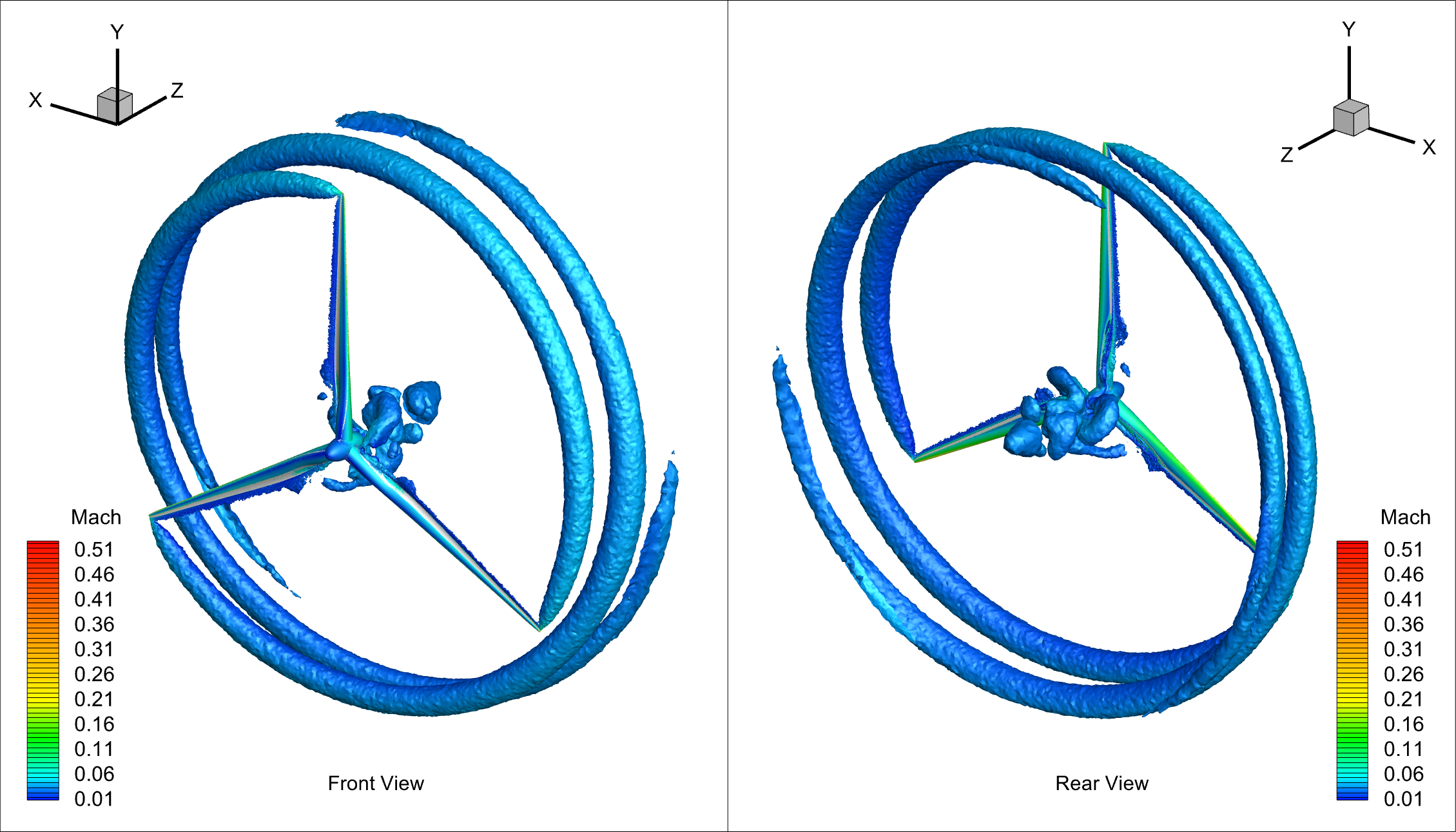
Fig. 6.10.8 Iso-surfaces of Q-criterion contoured by Mach number.

6.10.7. Sectional Loads on One of the Blades

To validate Flow360 results, sectional loads are examined in this section, with respect to the DTU CFD data. These sectional data were extracted from the flow solutions associated with one of the blades, that aligned with the positive direction of y-axis, for example, as shown in the above two figures. Following Flow360’s definitions, the forces shown in the following figures, and so on, are imposed on the turbine rotor by the fluid.

Spanwise distributions of the circumferential component of aerodynamic force are compared in Fig. 6.10.9. As expected, it was this force component that drove the rotor spinning around the positive z-direction. This is consistent with the \(C_{p}\) distributions shown above.

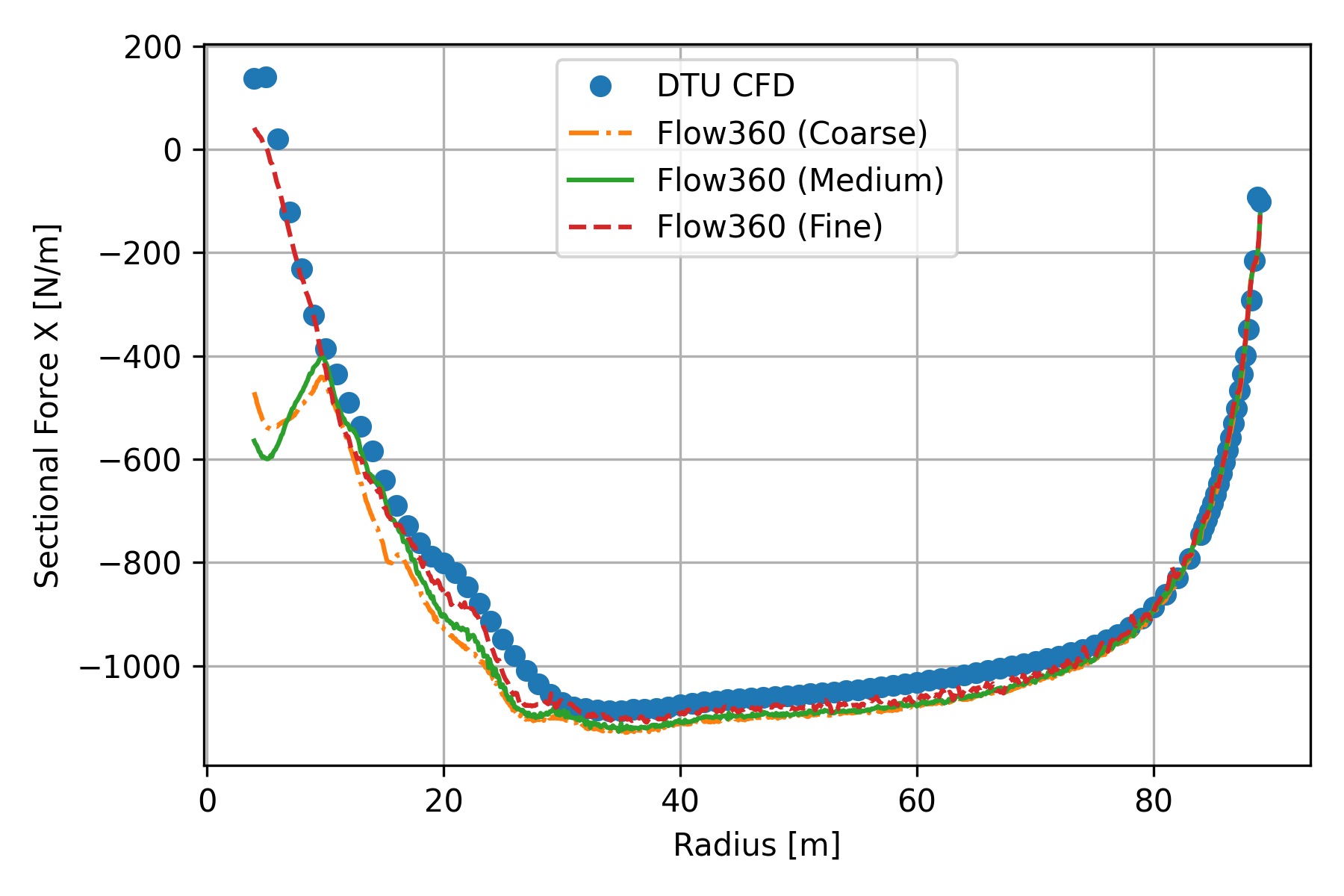
Fig. 6.10.9 Tangential force as function of radius.

Spanwise distributions of the axial component of aerodynamic force are compared in Fig. 6.10.10. Some discrepancies are present between Flow360 results and the reference at the outer blade, spanning from about 55 to 85 meters. In addition to the aforementioned differences in the turbine geometries, the differences between the current and reference simulation methodologies are likely contributing here, as summarized in Table 6.10.3. DTU results were computed on a structured grid with 14.1 million cells utilizing a pressure-based incompressible Reynolds-averaged Navier-Stokes (RANS) solver, where steady state simulations were performed with rotating effects analytically described as discussed, for example, by Troldborg et al and Johansen et al. Whereas, unsteady compressible DDES simulations were performed with Flow360, where a rotating mesh region was incorporated with sliding interfaces. It is suspected that weak compressibility effects may also contribute to such a discrepancy.

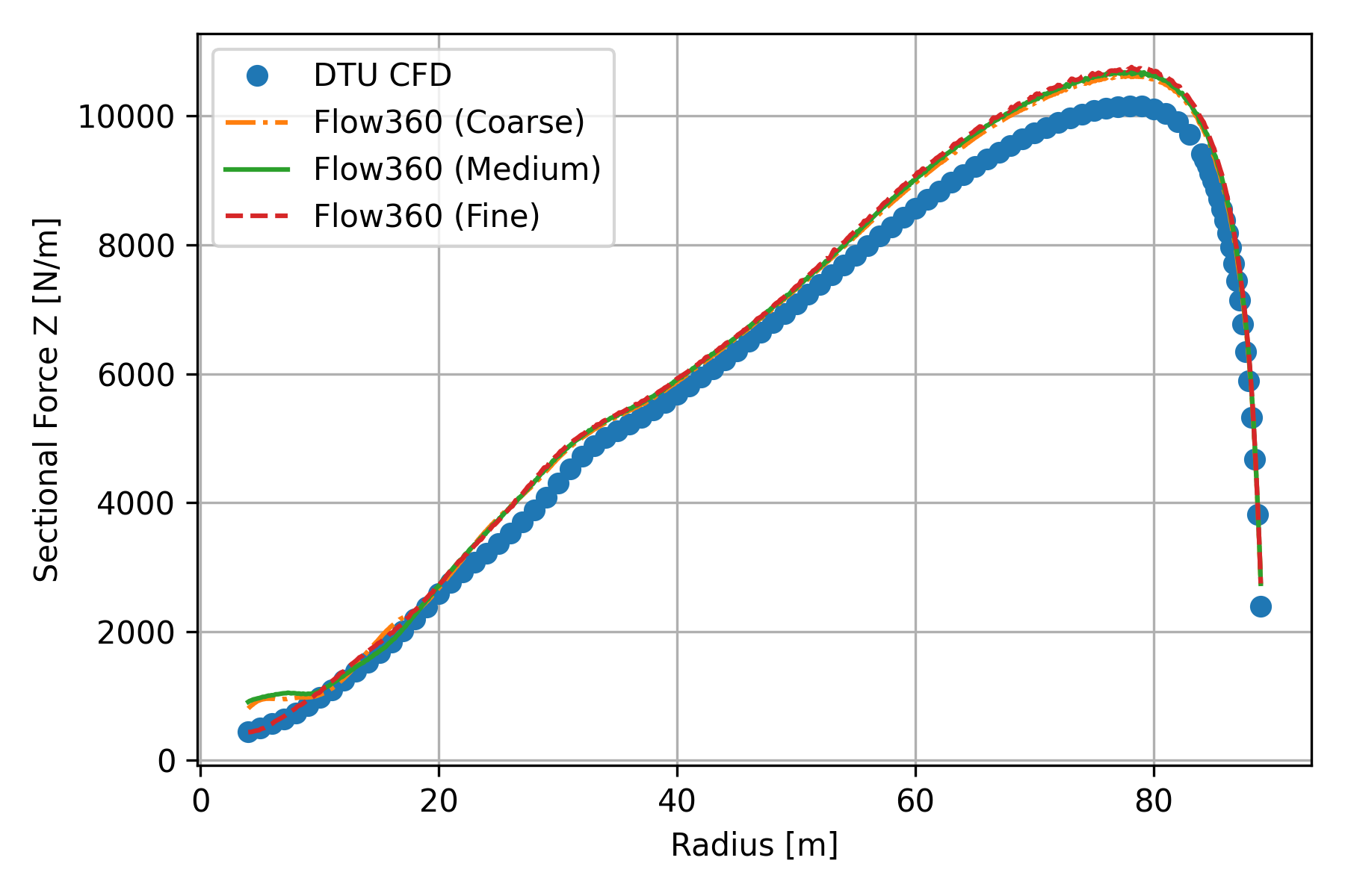
Fig. 6.10.10 Axial force as function of radius.

Table 6.10.3 Key flow solver features

Solver Features	Flow360	DTU EllipSys3D
Compressibility	Compressible	Incompressible
Grid Type	Unstructured	Structured
Simulation Type	Unsteady	Steady-state
Turbulence Model	DDES with SA	RANS with \(k-\omega\) SST
Boundary Layer Mode	Fully turbulent	Fully turbulent
Rotating Effects	Rotating Mesh via Sliding Interfaces	Moving Reference Frame

Local thrust coefficient, as defined by Eq.(6.10.1), are compared in Fig. 6.10.11. In the right hand side of Eq.(6.10.1), all quantities are dimensional. Here and in the next figure, a constant value of 3.4 meters was used for the reference chord length \(L_{chord,ref}\). Also, \(F_z(r)\) is the sectional axial force. As seen from the figure, there are relatively large differences near the blade root. This likely can be attributed to the presence of the elliptic fairing, together with grid density differences. However, these effects are marginal to the integrated power output.

(6.10.1)\[C_{thrust}(r) = \frac{F_z(r)}{\frac{1}{2} \rho_{\infty}(\omega \cdot r)^2 \cdot L_{chord,ref}} \cdot \frac{r}{R_{tip}}\]

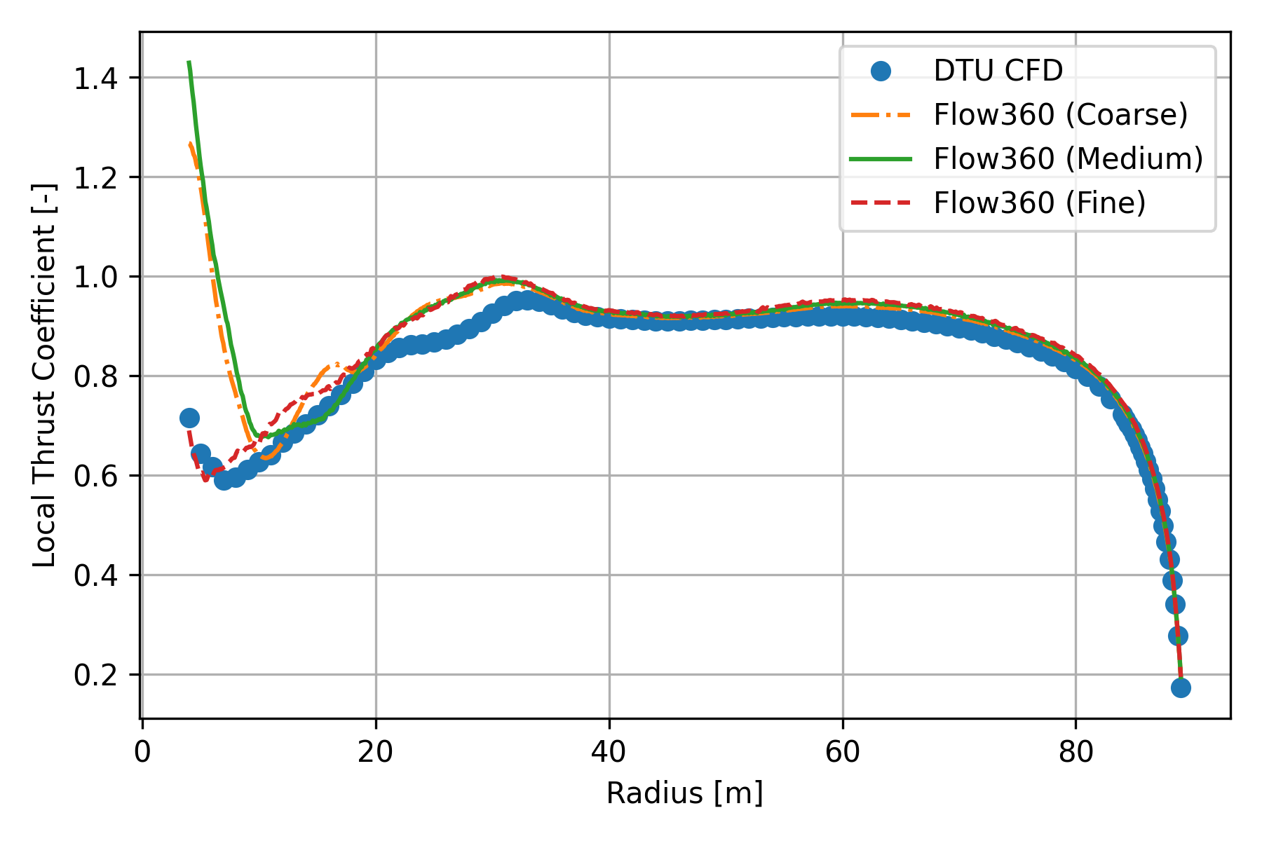
Fig. 6.10.11 Local thrust coefficient as function of radius.

Local power coefficients, as defined by Eq.(6.10.2), are compared in Fig. 6.10.12. Notably, in the definition, \(M_z(r)\) is the sectional axial moment. As seen from the figure, results agree well between current simulations on the three meshes and that of DTU CFD data, especially for spans greater than 10 meters. Contributions to the power output were decomposed into three segments along the blade, the inner (4 to 33 meters), the middle (33 to 61 meters) and the outer (61 to 89 meters) parts. The corresponding fractions to the total power were about 13%, 38% and 49%.

(6.10.2)\[C_{power}(r) = \frac{M_z(r)}{\frac{1}{2} \rho_{\infty}(\omega \cdot r)^2 \cdot L_{chord,ref}} \cdot \frac{r}{R_{tip}} \cdot \frac{\omega}{U_{\infty}}\]

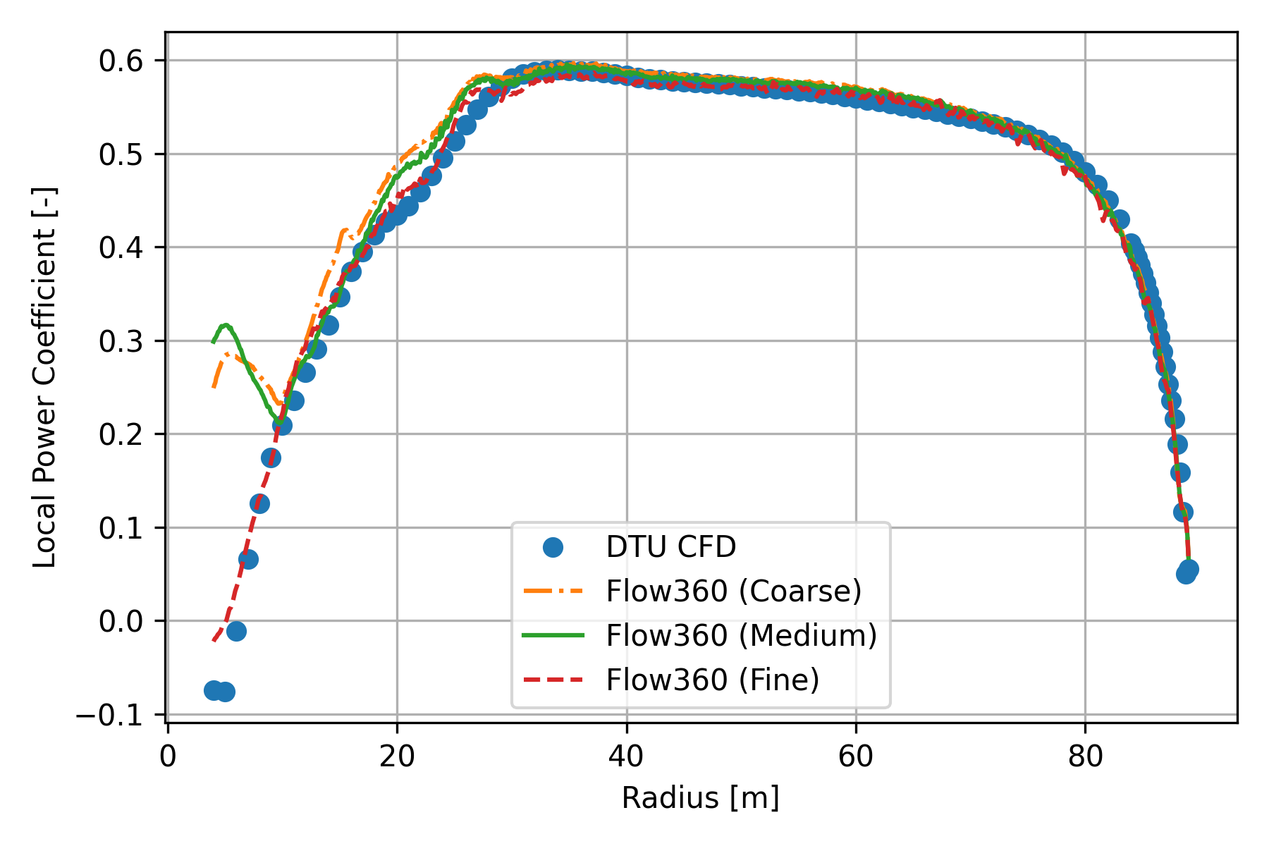
Fig. 6.10.12 Local power coefficient as function of radius.

6.10.8. Integrated Loads on the Entire Rotor

The integrated data of axial force and moment, as well as power output are summarized in Table 6.10.4. Flow360 results were averaged through the last one revolution. DTU results are also given in this table as references. Overall, reasonable agreement was achieved, with the maximum relative errors of 6.2% and 3.7% for integrated values of axial force and power, respectively.

Table 6.10.4 Integral axial force and moment coefficients, their dimensional values and the integrated power

Parameters	Units	Flow360 (Coarse)	Flow360 (Medium)	Flow360 (Fine)	DTU CFD
CFz	—	0.0158519	0.0157376	0.0156527	0.0149317
CMz	—	1.201E-03	1.211E-03	1.218E-03	1.174E-03
Fz	kN	1650.8	1638.9	1630.1	1555.0
Mz	N*m	1.115E+07	1.124E+07	1.131E+07	1.090E+07
Power	MW	10.3191	10.4047	10.4656	10.0885

For Flow360 results, it seems that these integrated performance parameters were asymptotically converging along with the grid refinements, as shown in Fig. 6.10.13. For the results computed on the coarse mesh, the relative errors of these dimensional quantities are all within 1.5%, with respect to those on the fine mesh. To reserve computational costs, off-design simulations were performed using the coarse mesh, as discussed in the next section with more details.

Fig. 6.10.13 Grid convergence. The lower x-axis is the number of grid nodes labeled as \(N\), and the corresponding upper axis shows the scale of the expected numerical error labeled as \(N^{-2/3}\). Dimensional values of axial force and mechanical power are shown in the upper and the lower frames, respectively.

6.10.9. Off-Design Performance

For validation and demonstration purposes, wind turbine operations were further simulated at off-design conditions. To limit engineering efforts without having to further reproduce more turbine geometries, four more off-design conditions with the same zero blade pitch angle as that operated at the rated condition were selected. The corresponding freestream wind speeds were 7.0, 8.0, 9.0 and 10.0 m/s. Also, as discussed above, the coarse mesh was used in these simulations.

Off-design sectional loads on one of the blades are shown in Fig. 6.10.14, Fig. 6.10.15, Fig. 6.10.16 and Fig. 6.10.17 for the spanwise distributions of tangential and axial forces, and local thrust and local power coefficients, respectively. For comparison, those of the rated power condition are also shown in these figures, together with the available DTU CFD data. As seen from these figures, overall agreement was well achieved. Notably, Flow360 results at the wind speed of 7.0 m/s are not shown in these figures for sectional loads, since the counterparts of DTU CFD data were not available.

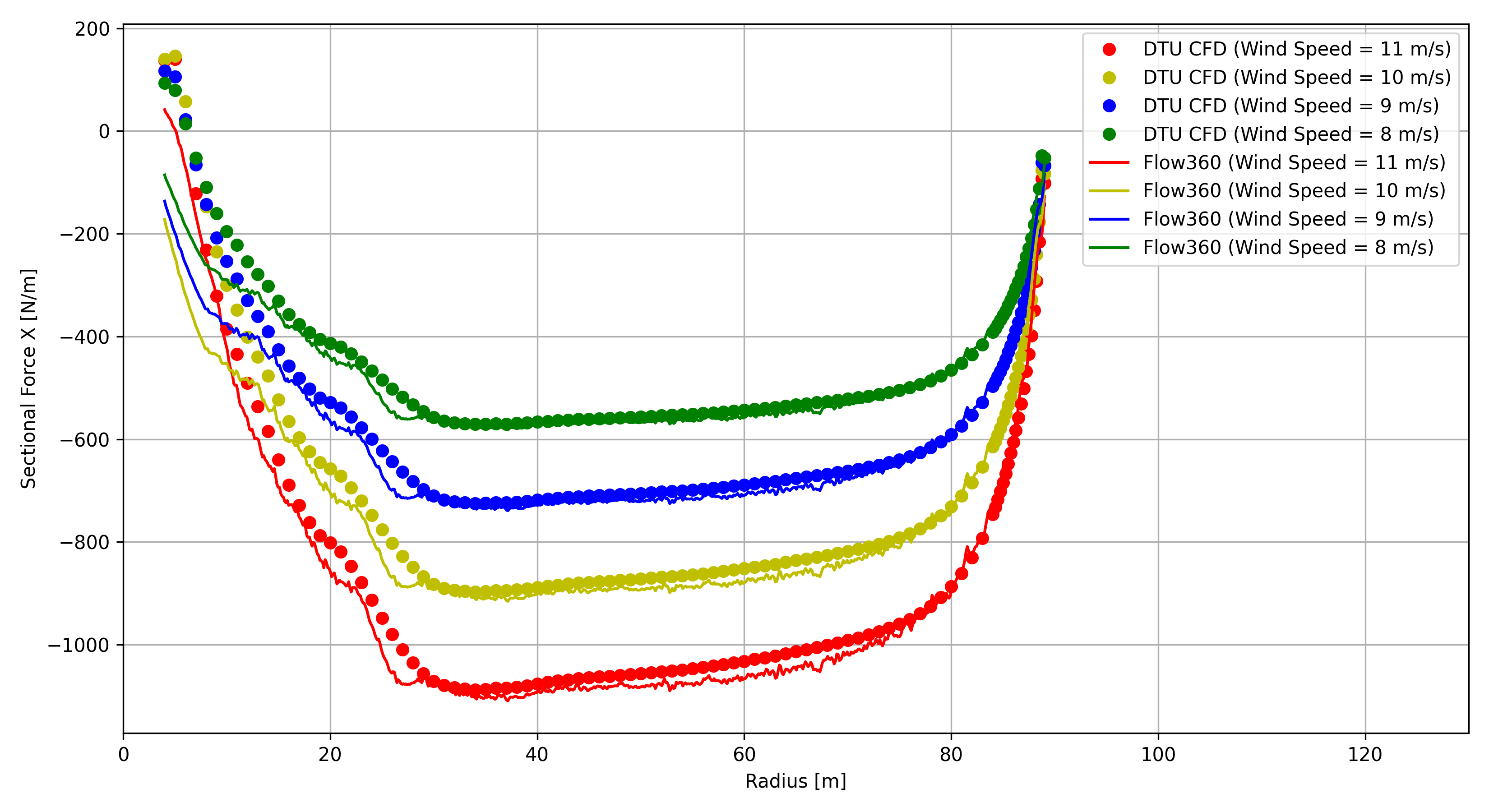
Fig. 6.10.14 Tangential force as function of radius.

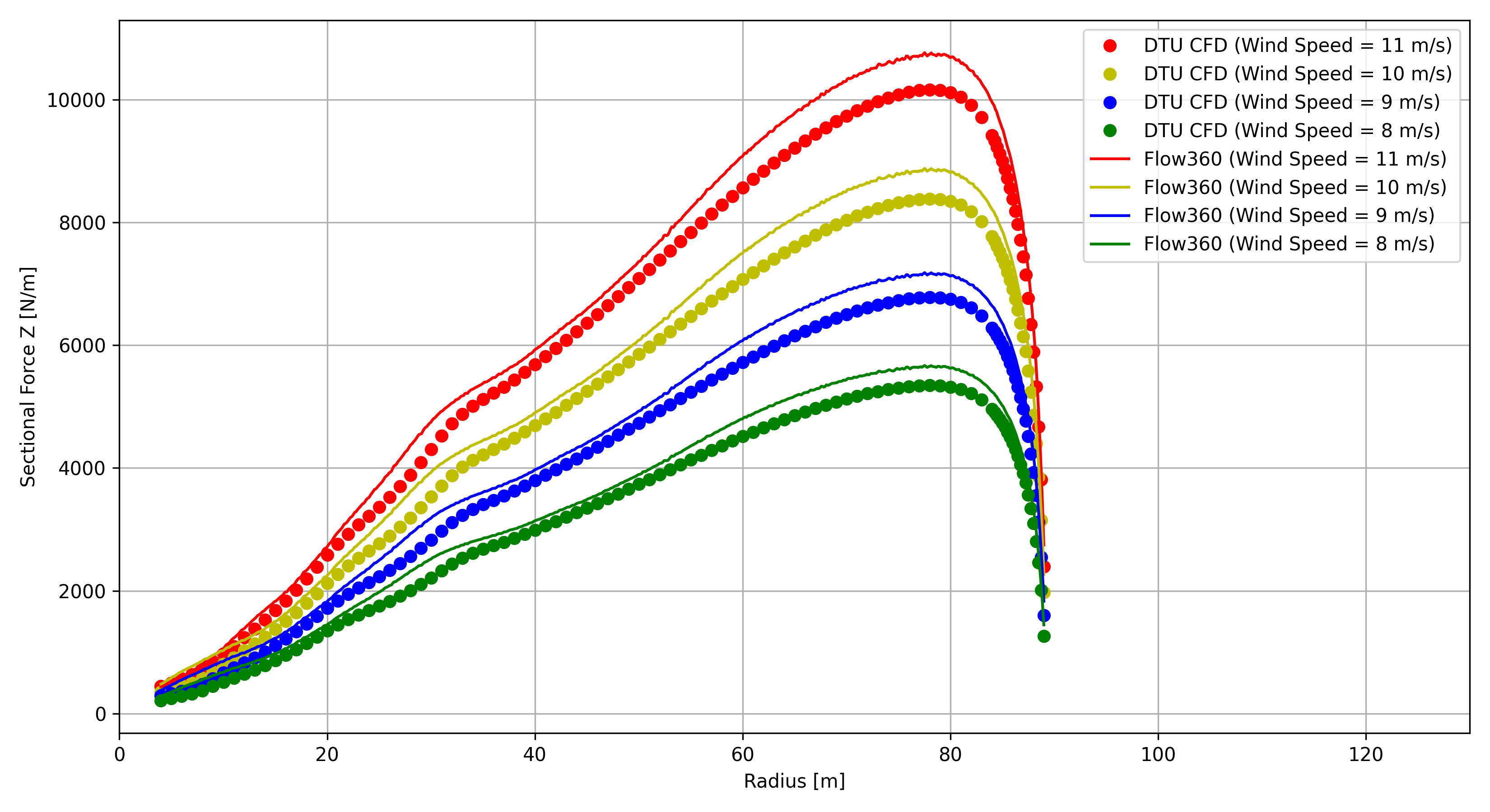
Fig. 6.10.15 Axial force as function of radius.

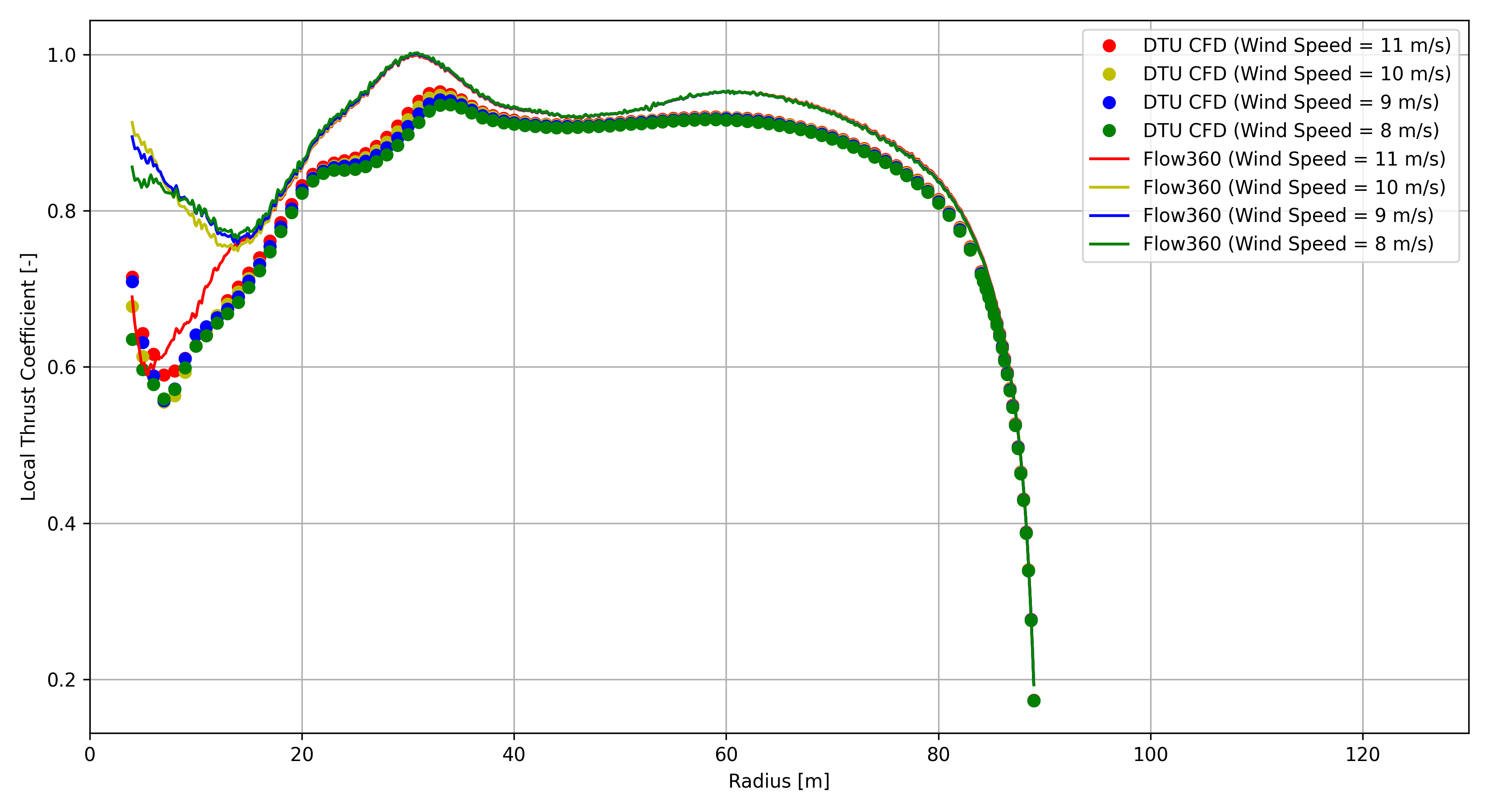
Fig. 6.10.16 Local thrust coefficient as function of radius.

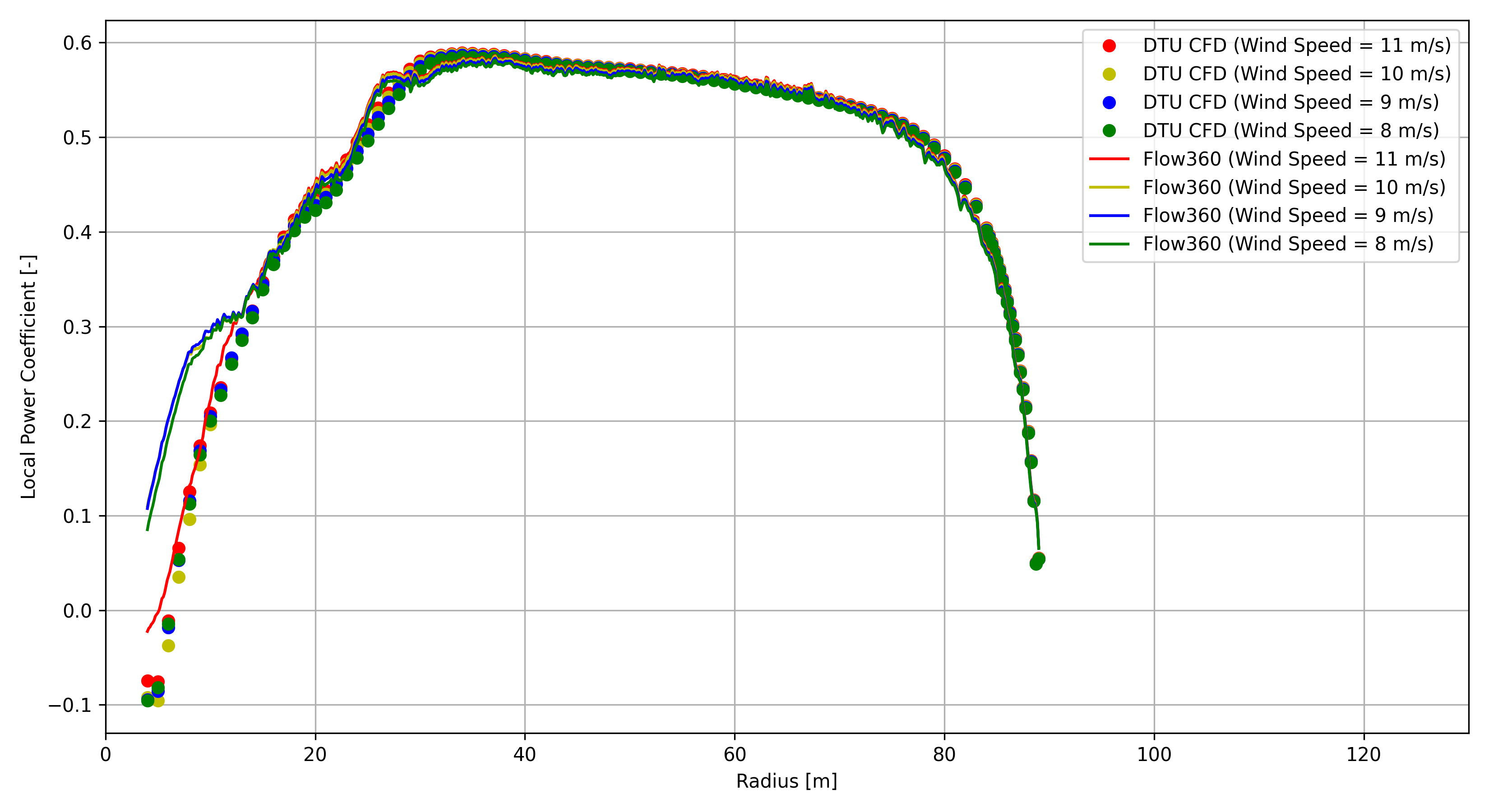
Fig. 6.10.17 Local power coefficient as function of radius.

The off-design key performance parameters, including integrated rotor power and thrust, and their coefficients, are summarized in Table 6.10.5. The definitions of these integral power and thrust coefficients are given in Eq.(6.10.3) and Eq.(6.10.4). Notably, Flow360 results were averaged through the last one revolution.

(6.10.3)\[C_P = \frac{Power}{\frac{1}{2} \rho_{\infty} (\pi \cdot R_{tip}^2) U_{\infty}^3}\]

(6.10.4)\[C_T = \frac{Thrust}{\frac{1}{2} \rho_{\infty} (\pi \cdot R_{tip}^2) U_{\infty}^2}\]

Table 6.10.5 Integrated rotor power and thrust and their coefficients as a function of wind speed.

Off-design Parameters
Wind Speed [m/s]	7.0	8.0	9.0	10.0	11.0
RPM	6.000	6.426	7.229	8.032	8.836
Flow360 (DDES)
Power [MW]	2.6140	3.9194	5.6119	7.7333	10.3191
Thrust [kN]	708.5	873.0	1104.5	1363.9	1650.8
Power Coefficient	0.498	0.500	0.503	0.505	0.507
Thrust Coefficient	0.945	0.892	0.891	0.891	0.892
DTU (RANS)
Power [MW]	—	3.8482	5.4966	7.5610	10.0885
Thrust [kN]	—	817.0	1036.6	1282.6	1555.0
Power Coefficient	—	0.491	0.493	0.494	0.495
Thrust Coefficient	—	0.834	0.837	0.838	0.840

Off-design characteristics are visualized in Fig. 6.10.18, where key performance parameters as summarized in the above table are shown in each frame with DTU CFD data. Flow360 predictions reasonably captured the simulated off-design performance . Off-design operations above the rated wind speed, 11m/s, can be expected to produce large flow separation from rotor blades. For these scenarios, DDES simulations would provide improved predictions with respect to RANS simulations.

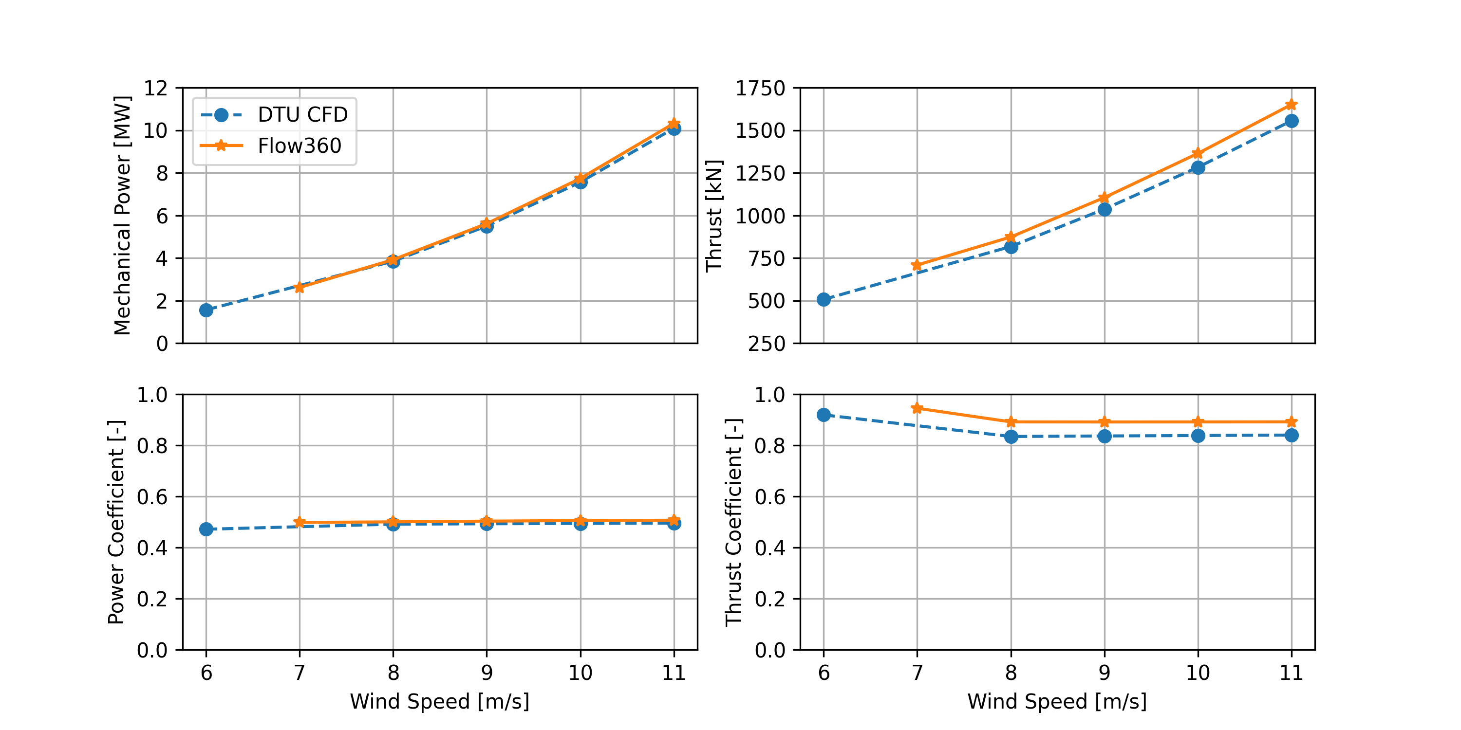
Fig. 6.10.18 Power and thrust and their coefficients as function of wind speed.