6.3. Blade Element Theory using the XV-15 rotor and the Flow360 Python API#
This tutorial aims to provide guidance for blade element theory (BET) simulations for each step of the process, from mesh generation, setting up the input files through to the simulation output and postprocessing. For a refresher on BET implementation, please see the Capabilities and Knowledge Base pages.
The example used for this tutorial will be the XV-15 rotor blade, which is also used for the sliding interface tutorial for rotating geometry simulations and the BET validation study. For this case we will be generating a simple wing. We will be using the automated meshing toolchain to generate the mesh. The configuration used in this tutorial is shown in Fig. 6.3.1 with a view from behind Fig. 6.3.5 and a side view Fig. 6.3.6.
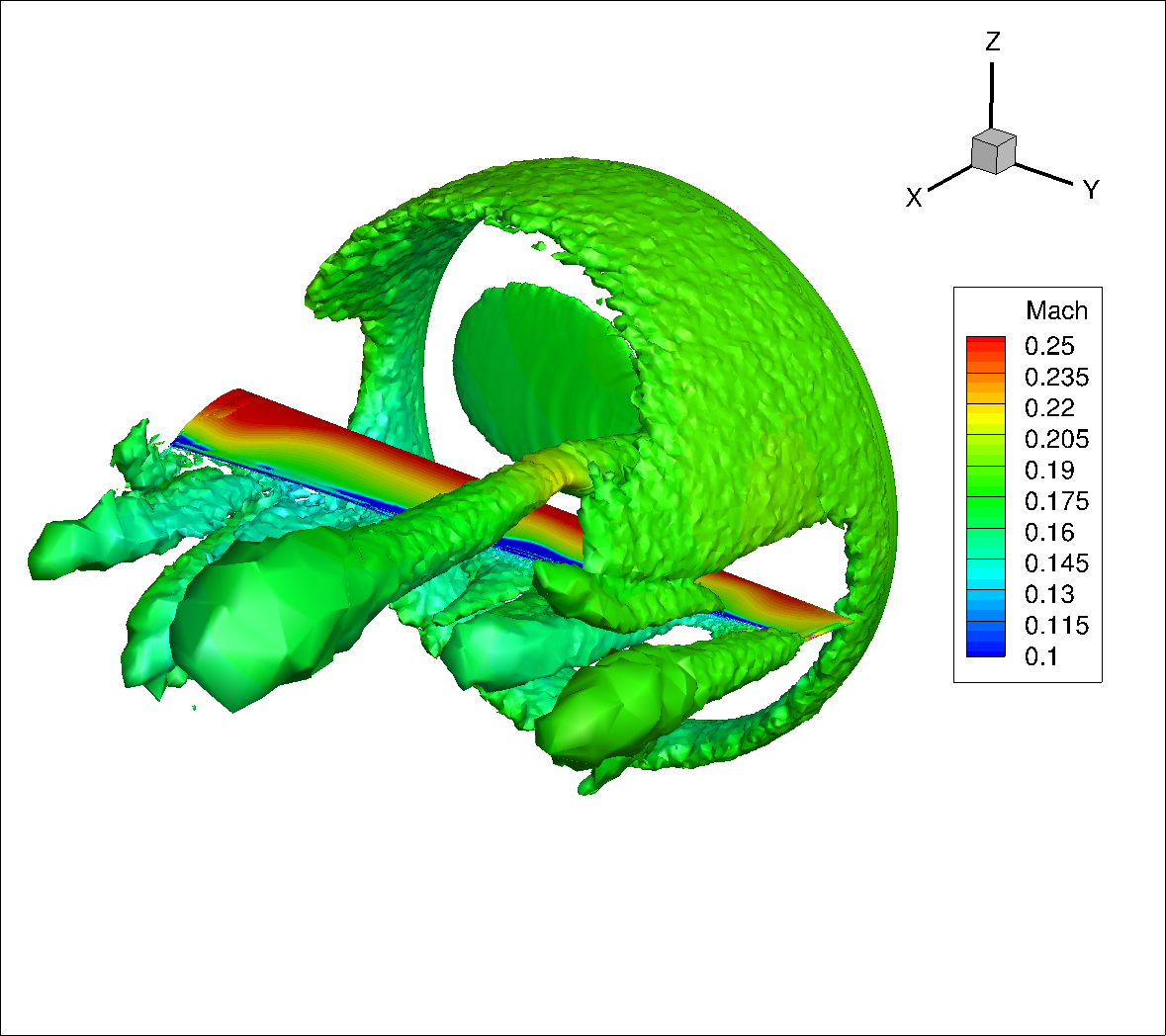
Fig. 6.3.1 BET tutorial case configuration visualized using Q-criterion contoured by Mach number.#
The tutorial will cover steady-state BET Disk simulations, but most of the explanations are also applicable to transient BET Line simulations.
Preprocessing#
The first section of the tutorial focuses on the geometry and mesh generation. The geometry model is built in Engineering Sketch Pad (ESP). The basic wing model CAD generation file we will use can be found in this BET_tutorial_wing.csm file. The surface and volume mesh parameters input files are discussed below.
This tutorial is meant to be used with the Flow360 Python API V2. All of the mentioned code will be using an import convention:
import flow360 as fl
Information on how to install the API can be found in Python API Guide.
In this tutorial the SI unit system will be used. To ensure correct handling of units, any code blocks where dimensional quantities are defined are enclosed witihin an appropriate with block.
with fl.SI_unit_system:
    ...
While the mesh can be generated manually using numerous meshing software, we will be using our automated meshing toolchain, which takes an ESP CAD model from a CSM file as an input. To use the automated meshing framework, at least one no-slip wall must be present in the simulation and should not cross-over the BET disk region. This can be either a hub for isolated rotor simulations or other vehicle elements such as a wing, tail etc.
For best practices and recommendations on how to generate meshes for BET simulations, please see the Knowledge Base.
The first step to setting up a pipeline is to define a project - an entity described in more detail in Cloud assets. In this case, the base asset will be a geometry:
project = fl.Project.from_geometry("./BET_tutorial_wing.csm", "BET_tutorial")
Accessing the geometry entities is done using the project.geometry attribute.
The BET disk should be placed in a specific refinement region. The XV-15 rotor blade has a radius of 3.81 meters, with the root of the blades at 0.3429 meters radius. Hence, following the recommendations mentioned above, our rotor disk refinement region should have the following dimensions:
Radially, we want the refinement region in the mesh to start at the disk center and go beyond 1.1 * the rotor disk radius to about 4.25 meters.
In the axial (thickness) direction, we should chose a value between 10% and 15% of the rotor radius; so we picked a 12% rotor radius value for the actual BET disk thickness in the simulation. Because the mesh refinement region should be slightly larger then the BET disk we will assume a value of 16% rotor radius thickness for the refinement region in the mesh. Hence, our refinement region will be 3.81 * 16% ~= 0.6m thick in the x-axis direction.
The extent and the placement of the refinement region is defined using a Cylinder object:
refinement_extent = fl.Cylinder(
                        name="refinement_extent",
                        inner_radius=0,
                        outer_radius=4.25,
                        height=0.6,
                        axis=(1,0,0),
                        center=(-2,5,0)
                    )
The spacing is defined as follows:
Since we want at least 20 nodes across the BET disk thickness we use a spacing of 0.02, which leads to 30 nodes across the refinement region in the mesh.
To maintain a good aspect ratio, the spacing in the radial direction is set to 0.03, leading to approximately \(\frac{4.25}{0.03} = 142\) nodes in the radial direction in the refinement region.
In the circumferential direction, we use a spacing of 0.06 leading to approximately 445 nodes along the perimeter.
For the hub we will implement it directly within the BET/AD formulation. This means defining polars and blade geometry all the way to the center of the propeller at r=0.
The object used to describe the refinement volume zone is an AxisymmetricRefinement, which in this case is defined as:
axi_refinement =  fl.AxisymmetricRefinement(
                    spacing_axial=0.02,
                    spacing_radial=0.03,
                    spacing_circumferential=0.06,
                    entities=[refinement_extent]
                )
The surface and volume meshing parameters are then defined as usually, more on meshing can be found in Automated Meshing.
geometry = project.geometry
farfield = fl.AutomatedFarfield(name="farfield", method="auto")
meshing = fl.MeshingParams(
        defaults=fl.MeshingDefaults(
            surface_max_edge_length=0.5,
            surface_edge_growth_rate=1.2,
            curvature_resolution_angle=30*fl.u.deg,
            boundary_layer_first_layer_thickness=1e-06,
            boundary_layer_growth_rate=1.15
        ),
        volume_zones=[
            farfield,
        ],
        refinements=[
            fl.SurfaceEdgeRefinement(name="edge_refinements1",
                                     entities=[geometry["wingLeadingEdge"],
                                               geometry["wingTrailingEdge"]],
                                     method=fl.HeightBasedRefinement(value=0.0003)),
            fl.SurfaceEdgeRefinement(name="edge_refinements2",
                                     entities=[geometry["rootAirfoilEdge"],
                                               geometry["tipAirfoilEdge"]],
                                     method=fl.ProjectAnisoSpacing()),
            fl.SurfaceRefinement(name="tip_refinement",
                                 faces=[geometry["tip"]],
                                 max_edge_length=0.01),
            fl.UniformRefinement(name="refinement", spacing=0.1,
                                 entities=[
                            fl.Cylinder(
                                name="refinement_cylinder",
                                outer_radius=4.4,
                                height=5,
                                axis=(1,0,0),
                                center=(0,5,0)
                            )
            ]),
            axi_refinement
        ]
    )
Note
In the previous steps, we configured all the parameters for mesh generation—an integral part of the workflow you’ll submit at the end of this tutorial . Below, you’ll find screenshots of the final mesh.
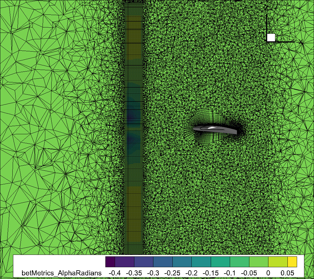
Fig. 6.3.2 Slice of the volume mesh at wing mid-span (y=5), showing the BET disk refinement region in the axial direction. Notice the structured axi_refinement refinement region within an unstructured region to better capture the physics of interest.#
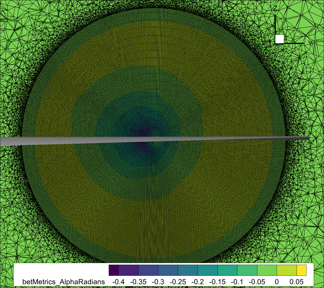
Fig. 6.3.3 Slice of the volume mesh at the BET disk center (x=-2), showing the BET disk refinement region in the radial and azimuthal direction.#
Flow360 BET Configuration#
The next step is to define BETDisk object to be used as a volume zone in the SimulationParams object.
Rotor geometric information#
Rotor geometric information is defined using the entities attribute which takes a list of Cylinder objects that describe the regions where the BET formulation will add energy to the flow to simulate the propeller. Within each Cylinder object there are following parameters to define:
outer_radiusshould be set to the rotor radius.heightdescribes rotor’s thickness which was chosen to be 12% of the radius.axisdescribes the thrust axis of the rotor.centerdescribes the center of rotation of the rotor.
Additionaly other attributes describe the rotor shape:
number_of_bladesdescribes the amount of blades in the rotor.rotation_direction_ruleis used to define the thrust directon.blade_line_chordis used only for time accurate blade line simulations. When doing steady state BET disk simulation, it can be ignored or set to 0.tip_gapThe BET disk formulation has a tip loss correction to account for 3D flow effects near the tip of the blade. If some external feature (duct, shroud, cowling, nacelle, etc.) affects that 3D tip loss, the user can vary thetip_gapparameter to decrease the amount of 3D tip losses all the way to 0 if desired.twistsis a list ofBETDiskTwistobjects specifying the twist as a function of radial location.chordsis list ofBETDiskChordobjects specifying the blade chord as a function of the radial location.
Rotor performance information#
The performance data consists of the omega parameter being the rotation speed, the mach_numbers, reynolds_numbers and alphas lists defining the values for which the aerodynamic coefficients are defined and sectional_polars and sectional_radiuses lists defining the performance of the cross sections included in the rotor.
Though entering the profiles aerodynamic information manually is possible and described in the BETDiskSectionalPolar class documentation, such approach is not recommended. Instead it is encouraged to generate the data in one of the common formats: C81, XFOIL, XROTOR, DFDC and use a dedicated constructor to translate the data from the file to the BETDisk object.
Rotor outputs#
The rotor outputs are defined using two parameters:
n_loading_nodesis the number of spanwise nodes that will be used to report propeller sectional loads Ct vs span and Cq vs span values in the bet_forces_v2.csv BET output file.chord_refis used to display the resulting Ct and Cq values on the blade’s 2D section. It is used to calculate the dimensional thrust and torque values. The blade MAC is typically an appropriate value.
Defining the Python object#
Finally we define the BETDisk volume model. In this tutorial the XROTOR file is used to define the aerodynamic data. The file can be downloaded here.
Since we want to replicate the airplane mode, blade pitch 26° condition discussed in this validation study, we need to have the following run conditions:
Tip Mach Number = 0.54.
RPM = 460 (to get the tip mach values above).
Advance ratio (defined as inflow speed over tip speed)= 0.337 which means the inflow Mach = 0.182.
Cylinder.axis: In this case it is important to note that the X axis points towards the aft of the wing while we want the thrust to be forwards in X, hence ourCylinder.axismust be [-1,0,0] to have a thrust axis pointing forward in X. See this documentation section.rotation_direction_rule: can be defined using a right-handed or left-handed coordinate system. For more information on the rotation direction see the following entry in our knowledge base. In the object below you can see we choserightHand.chord_ref: this value is only used to post-process the sectional loads in the bet_forces_v2.csv file. It is required as an input but is only needed if you want to redimensionalize the extracted local slice Cl and Cd values into dimensional values. In this tutorial we chose the mean propeller chord to set"chord_ref": 0.3556.tip_gap: this can be used to introduce the presence of a duct/shroud through a tip loss effect, see more in the BET knowledge base. Here we use the default (no effect) by removing the parameter.
With such parameters the object is constructed:
bet_file = fl.XROTORFile(file_path="xv15_rotor_26deg.xrotor")
bet_disk = fl.BETDisk.from_xrotor(
    file=bet_file,
    rotation_direction_rule="rightHand",
    omega=460*fl.u.rpm,
    chord_ref=0.3556,
    n_loading_nodes=20,
    entities=[
        fl.Cylinder(
            name="bet_disk",
            outer_radius=3.81,
            height=3.81*0.12,
            axis=(-1,0,0),
            center=(-2,5,0)
        )
    ],
    length_unit=fl.u.m,
    angle_unit=fl.u.deg,
)
Running the case#
The last parameters to define are some standard ones required to run any simulation.
operating_condition=fl.AerospaceCondition.from_mach(mach=0.182, alpha=5*fl.u.deg)
models = [
    fl.Freestream(surfaces=farfield.farfield),
    fl.Wall(surfaces=[geometry["wing"], geometry["tip"]]),
    fl.SlipWall(surfaces=[farfield.symmetry_planes]),
    fl.Fluid(
        navier_stokes_solver=fl.NavierStokesSolver(absolute_tolerance=1e-10),
        turbulence_model_solver=fl.SpalartAllmaras(absolute_tolerance=1e-10)
    ),
    bet_disk
]
time_stepping=fl.Steady(max_steps=20000)
outputs = [
    fl.VolumeOutput(
        output_fields=[
            "primitiveVars",
            "betMetrics",
            "qcriterion"
        ]
    ),
    fl.SurfaceOutput(
        output_fields=[
            "primitiveVars",
            "Cp",
            "Cf",
            "CfVec"
        ],
        surfaces=[geometry["wing"], geometry["tip"]]
    )
]
Finally all of the building blocks come together to form a SimulationParams object.
params = fl.SimulationParams(
    meshing=meshing,
    operating_condition=operating_condition,
    models=models,
    time_stepping=time_stepping,
    outputs=outputs
)
With SimulationParams the only thing left to do is to run the case:
project.run_case(params=params, name="BETTutorial")
Output and postprocessing#
The first thing to check when postprocessing a simulation is its convergence. Getting the Nonlinear Residuals to below 1e-10 is the target for simulation accuracy. Figure Fig. 6.3.4 below shows the convergence plot for this simulation, which achieves our convergnece target.
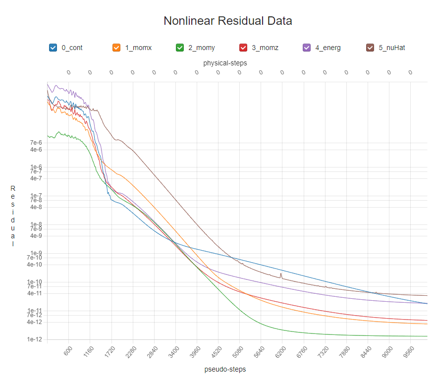
Fig. 6.3.4 BET Disk run convergence showing very good 7 orders of magnitude residual reductions. To see the convergence plot, navigate to web app (flow360.simulation.cloud) and open your latest project, navigate to analysis tab.#
As mentioned in our quickstart section, To download the surface data and the entire flow field, use the following command lines, respectively:
case = project.get_case()
results = case.results
    results.download(
        nonlinear_residuals=True,
        surface=True,
        volume=True,
        overwrite=True
    )
Once downloaded, you can postprocess these output files in either Tecplot or ParaView. You can specify the exported data you want in the outputs section of the SimulationParams object.
If the BET disk configuration is simulated for the first time, it is useful to examine the flow field solution, with a particular emphasis on the BET disk metrics. Flow360 outputs BET specific volumeOutput metrics to help evaluate the BET solution. This helps to make sure that the BET disk input is correct and that the volumetric mesh refinement regions are aligned with expectations. For example, by looking at the contours of the BET metric betMetric_AlphaRadians, which is zero outside the BET disk, we can see in Fig. 6.3.2 and Fig. 6.3.3 above that, as expected, the BET disk in the simulation is slightly thinner and slightly smaller in radius than the refinement region.
Example visualizations of the BET disk angle of attack are shown in Fig. 6.3.5 and Fig. 6.3.6 below.
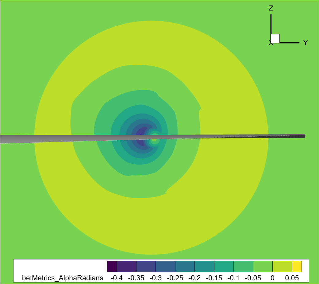
Fig. 6.3.5 View from behind of BET disk in front of the wing. Visualized using the calculated local blade angle of attack. Notice that this simulation was done with AoA= 5°, hence we have the expected asymmetry in the local blade angle of attack. The visualisations were generated using the web app (flow360.simulation.cloud), they can be accessed by opening the last project and navigating to analysis, and then visualisation tab.#
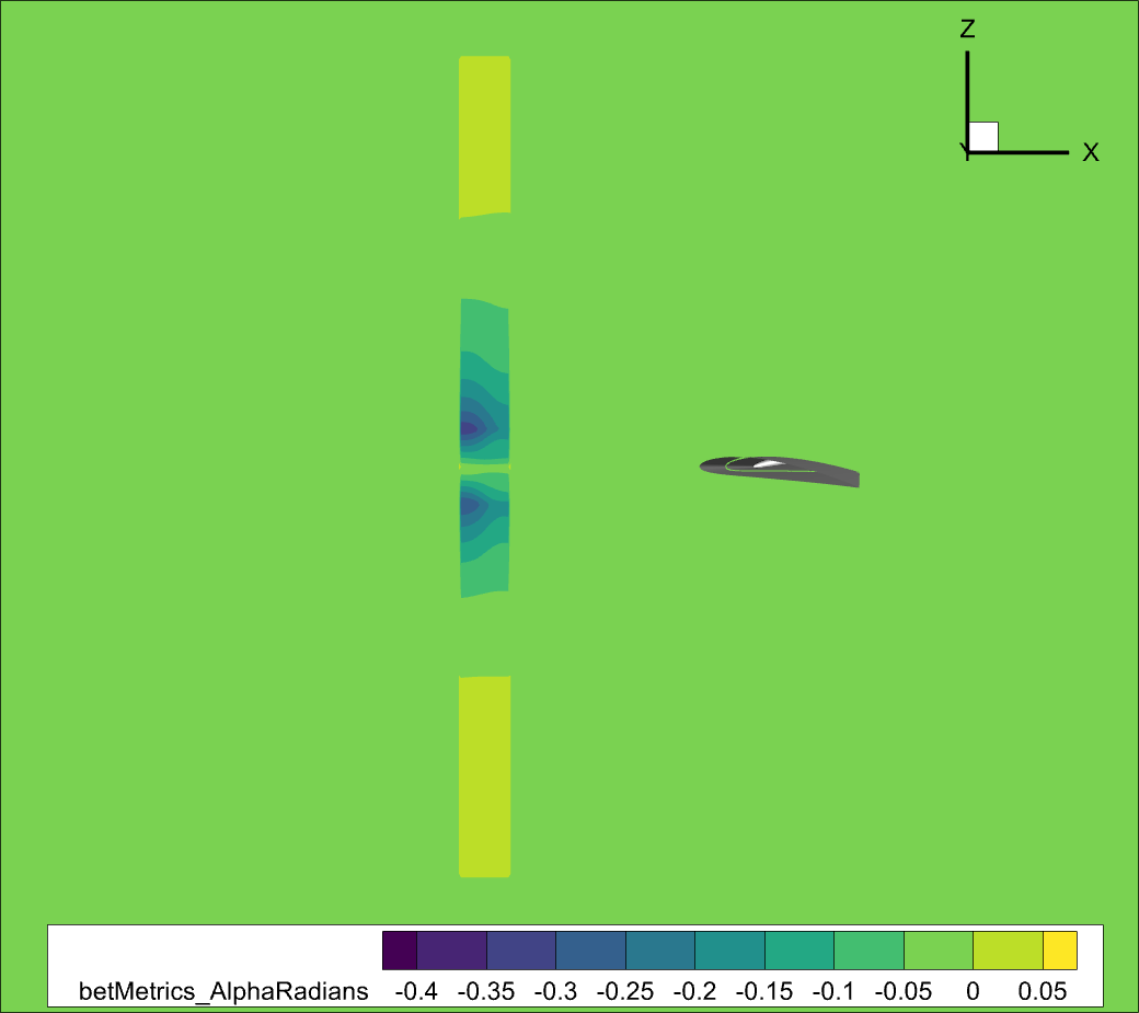
Fig. 6.3.6 Side view BET disk in front of the wing. Visualized using the calculated local blade angle of attack.#
The qcriterion output is a very good method for visualizing vorticity and generally better understand where propeller wakes are flowing. As we can see in Fig. 6.3.1 the vortices being shed by the BET disk are clearly visible. Please note that as the BET disk generates a smooth shear layer once past the initial sharp wake contraction, it is not very well resolved in this relatively coarse mesh.
For BET simulations, the Forces and Moments (F&M) values seen in the WebUI as well as reported in the total_forces_v2.csv and surface_forces_v2.csv files only include forces on no-slip walls present in the simulation, they do NOT include the BET disk F&M.
The BET disk F&M are only located in the bet_forces_v2.csv file. To obtain dimensionalized values of the Forces and Moments the to_base method can be used.
results.bet_forces.to_base("SI")
results.bet_forces.to_file("bet_forces_in_SI.csv")
In order to get the forces on the whole vehicle, care must be taken to combine the components from the no-slip walls with the components from the BET Disk.
For more details on how to post process BET forces, please see this validation study.