7.6. Fixing Divergence Issues#
In the event of a diverged cases, this section provides recommendations that may help to address the issue.
General Recommendations#
When a case status indicates diverged, which means either the Navier-Stokes solver or turbulence solver has diverged, it is necessary to identify the source of divergence.
Check the arguments of the case configuration file and make sure values for the flow conditions and boundary conditions are properly assigned. The divergence issue could be due to an unintended input, for instance, assigning value of
muReftoReynoldsby accident.Verify that there are no obvious problems with the mesh. For example, confirm that there are no negative volume cells and that boundary conditions are correctly assigned. Any obvious mistake that can be detected by a quick a review and is related to the mesh can potentially cause divergence.
Find the location of divergence. In the actions section in front of each case, by selecting the download button, logs/flow360_case.user.log file can be downloaded.
Investigating the Location of Divergence#
At the end of the “flow360_case.user.log” file, the user can find the error message for a diverged case: :code`(ERROR 3000) Solver is diverged`. A few lines above this message, users can see which solver is diverged: Navier-Stokes solver or turbulence solver.
When the Navier-Stokes solver diverges for a case, in the lines preceding this message, the minimum values for \(density\) (i.e., min rho in the user log) and \(pressure\) (i.e., min p in the user log), and maximum value for \(velocity\) (i.e., max Umag in the user log) are written.
At the end of each line, grid coordinates are printed following xyz=. The coordinates associated with nonphysical values, negative min rho for example, indicate the location of divergence. Similarly, when the turbulence solver diverges, grid coordinates for the maximum residual of the turbulence model can be taken.
For example, user-log message for a diverged case is shown below.

Fig. 7.6.1 User-log example showing the location of min rho where the Navier-Stokes solver is diverged.#
The next step is to check the mesh around the grid coordinates taken from the flow360_case.user.log file and make sure there is no obvious problem around those coordinates. Often an abrupt change in the area ratio or aspect ratio can cause divergence. It is recommended to maintain a smooth transition between small and large cells, specifically where 3D flow in the domain could be abruptly changing. Please refer to best practices for building the mesh.
It is also possible to find the location of min/max values on the WebUI. In the MinMax tab, \(min\_rho\), \(min\_p\) and \(max\_umag\) variations are shown with respect to pseudo steps. For example, by clicking on the \(min\_rho\) plot, a table appears that shows the value and location of the selected point. In the case of divergence, clicking on the last pseudo step plotted will present the location of divergence.
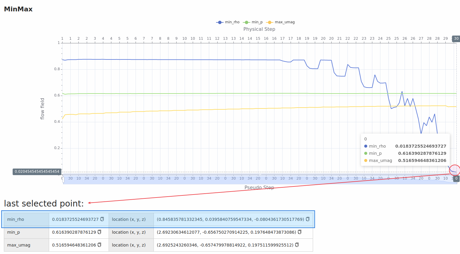
Fig. 7.6.2 Web-UI example showing the location of min rho where the Navier-Stokes solver is diverged.#
Steady Simulations#
When running a steady simulation, divergence may occur because of improper tuning of the CFL value. The CFL number defines the rate by which the information is traveling across a computational grid. The greater the value of CFL, the faster convergence can be achieved. However, the allowable CFL number depends on the characteristic size of the mesh cell. A CFL number that is too large for the mesh and flow can cause the linear solver to diverge. When a steady case is diverging and the cause of divergence is none of the above-mentioned issues in general recommendations, please follow the instructions below.
Checking the user log#
The first step is checking the flow360_case.user.log file and making sure that the simulation runs for at least a few pseudo-steps before it diverges. If a simulation immediately diverges without any iterations, please review guidance in general recommendations. Often a very small initial height in the boundary layer could require the initial CFL value to be less than 1 in order to be able to start a simulation and to avoid immediate divergence. In that case, ramping the CFL value can be used to avoid lengthy iterations to achieve proper residual drop for a steady simulation.
Reducing the initial value of CFL number#
If a simulation starts and runs for some pseudo-steps and then it diverges, as an initial test, users can reduce the initial value of the CFL number to a small value and see if this affects the iteration at which the divergence happens. If the iteration at which the divergence happened changes by decreasing the initial value of the CFL number, this means that the CFL number for this mesh and case configuration must be tuned. Tuning the initial CFL number for a fine mesh can be time consuming. It is recommended to decrease the initial CFL value substantially to help ensure that the early divergence is avoided. Testing initial CFL reductions with a coarse mesh can help as well.
Increasing the ramp step#
If the simulation diverges after the final CFL number is achieved, then the ramping step can be increased further to delay the iteration by which the final value of the CFL number is achieved to avoid divergence.
Decreasing the final value of CFL number#
If the simulation starts and runs for some pseudo-steps and diverges when the value of the CFL number is being increased toward the end of the ramping step, and increasing the ramping steps doesn’t help to avoid the divergence, the final value of the CFL number can be decreased to avoid divergence.
Improving convergence when residuals are stalling#
If the above CFL recommendations have been addressed and the residuals remain “stalled” (i.e., no longer reducing), locally increasing the mesh resolution in areas of high gradients can help to obtain better convergence. Another possible option in this instance is to run an unsteady simulation until a stabilized solution is achieved with improved convergence.
Avoiding divergence through the use of adaptive CFL#
Instead of using the ramp approach, where the initial, final and rampSteps need to carefully be chosen to avoid divergence, the user can switch to the adaptive algorithm, which automatically adjust the CFL number based on the linear residuals (see more in the adaptive CFL knowledge base). To demonstrate through an example, we use the ONERA quick-start example with an increase in alpha to 10 degrees, which makes it a more complex case that is more susceptible to divergence than the baseline case. For the ramp simulation we used a ramping of CFL from 5 to 200 over 100 ramp steps, which diverges after 110 pseudo steps. On the other-hand the adaptive CFL with default settings, manages to converge this simulation, with the residuals convergence and CFL values during the simulation shown in Figures Fig. 7.6.3-Fig. 7.6.6. It must also be noted that the adaptive CFL value at the end of the simulation is approx. 240 which is above the final value for the ramp simulation.
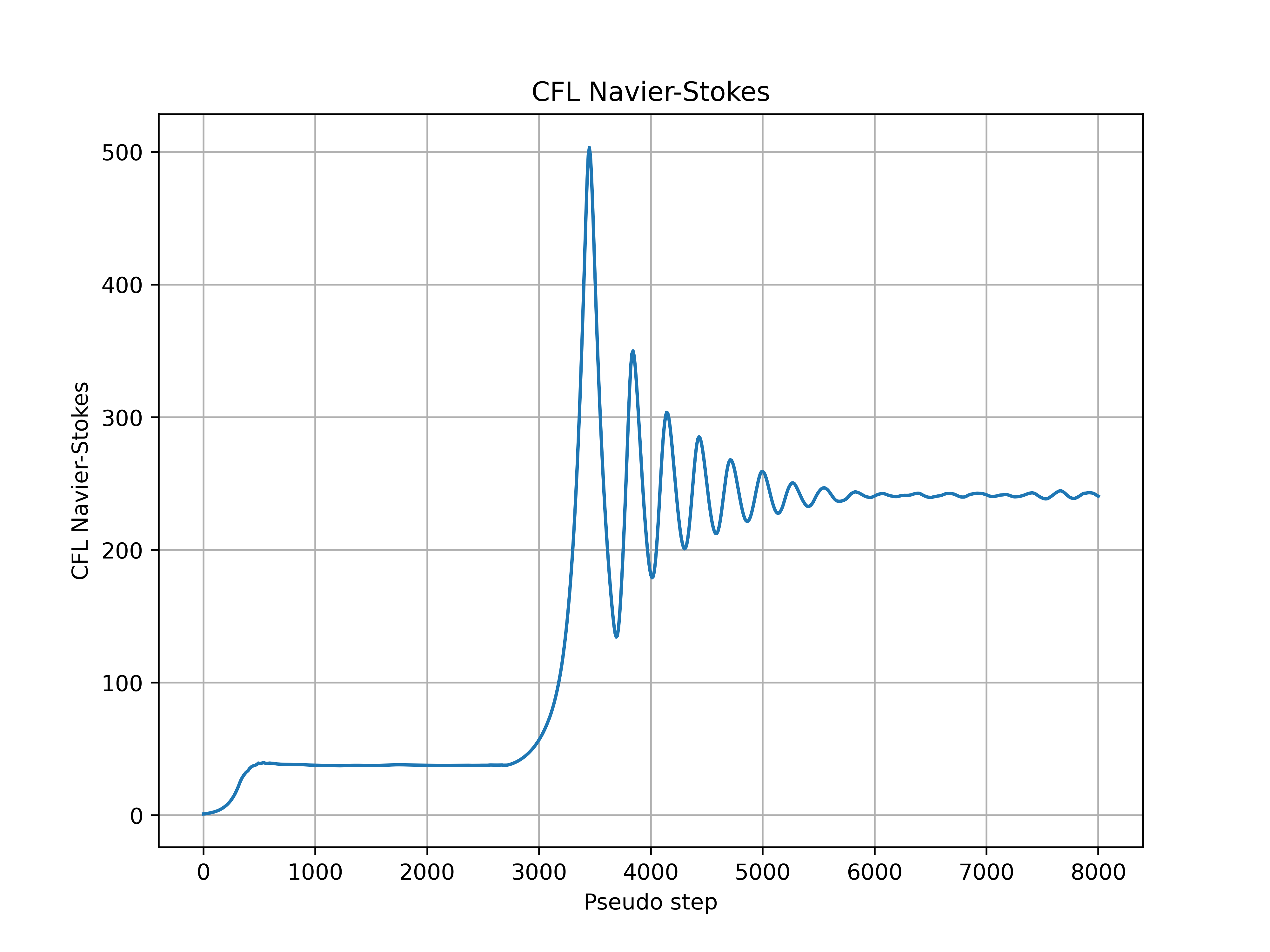
Fig. 7.6.3 Navier-Stokes CFL number during the simulation for the ONERAM6 wing at 10 degrees alpha.#
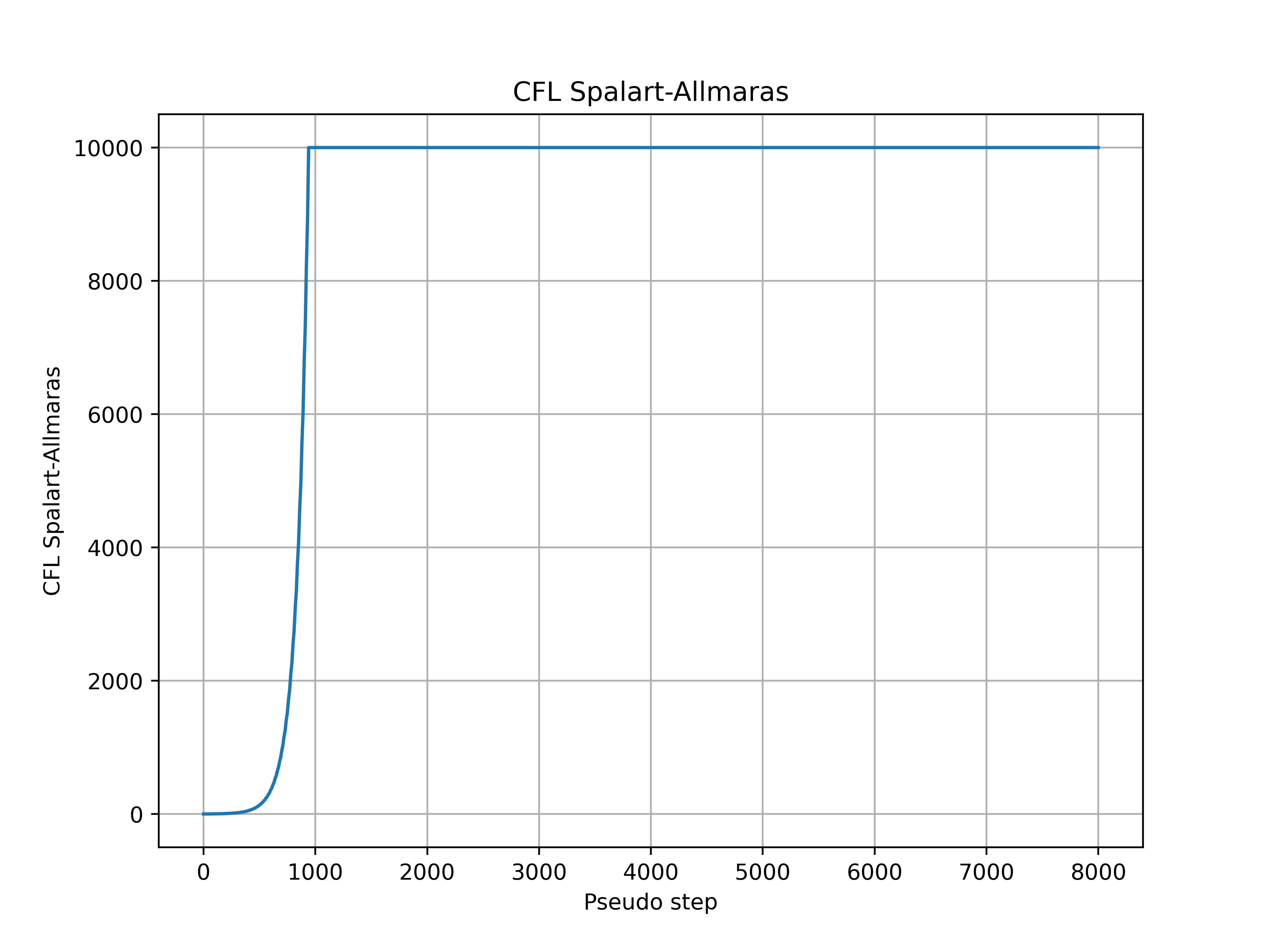
Fig. 7.6.4 Spalart-Allmaras CFL number during the simulation for the ONERAM6 wing at 10 degrees alpha.#
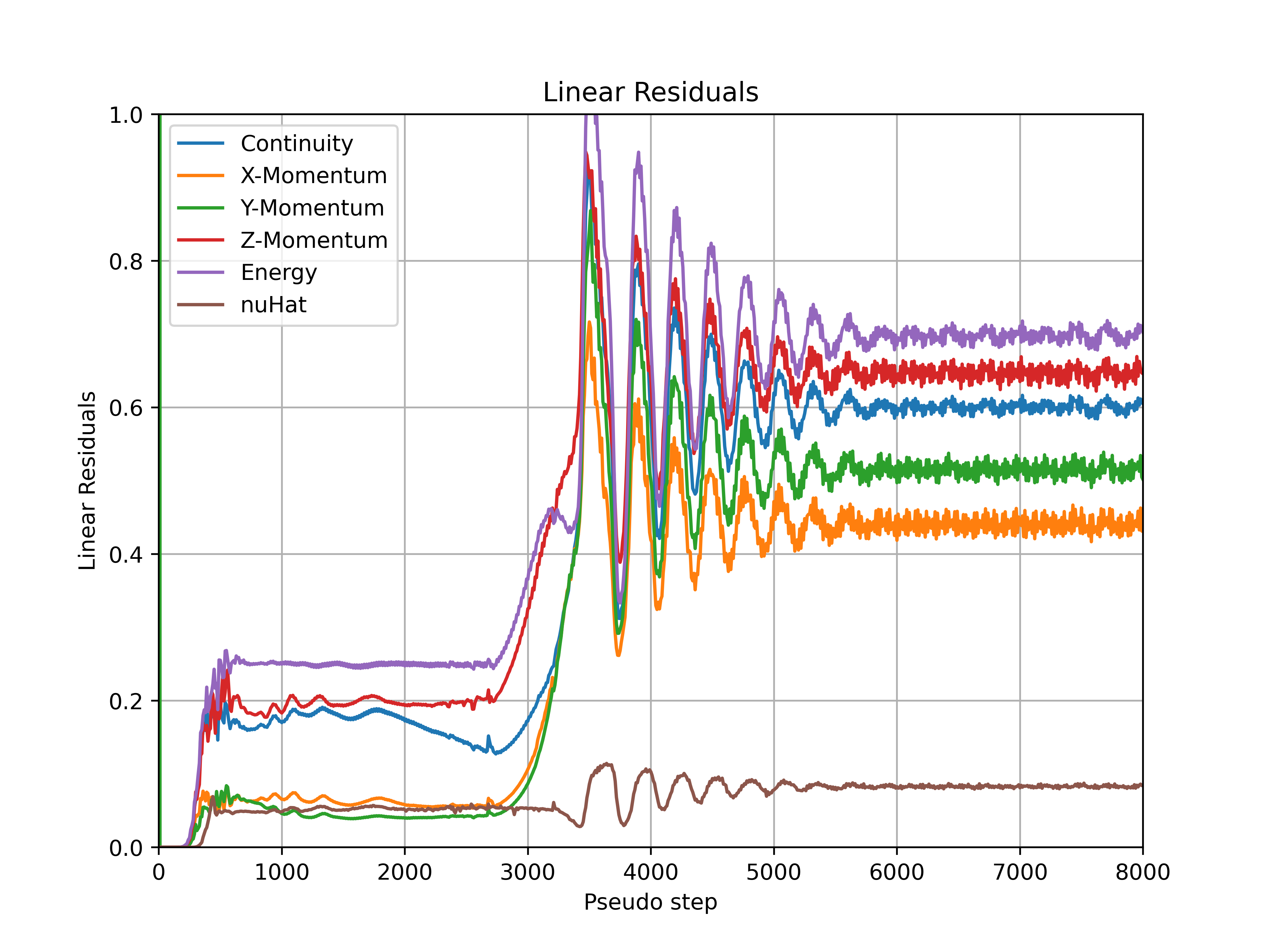
Fig. 7.6.5 Convergence of the linear residuals during the simulation for ONERAM6 wing at 10 degrees alpha.#
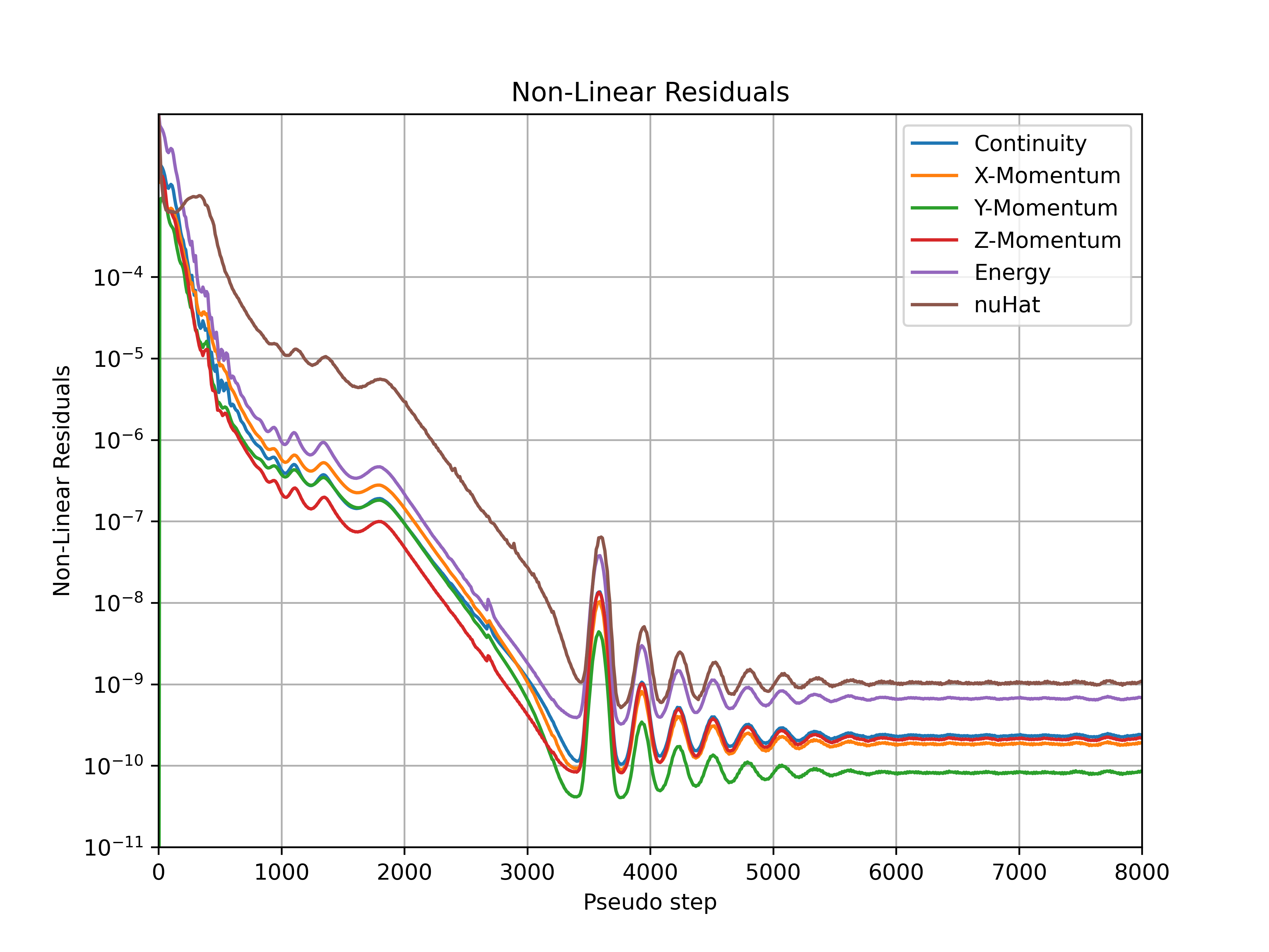
Fig. 7.6.6 Convergence of the nonlinear residuals during the simulation for ONERAM6 wing at 10 degrees alpha.#
Unsteady Simulations#
When running an unsteady simulation, and the case is diverged, please first check the general recommendations and make sure that none of the issues referred is the reason for divergence.
It is recommended to have residuals drop at least two orders of magnitude within each physical step. An example of unsteady residuals are shown in the below figure.
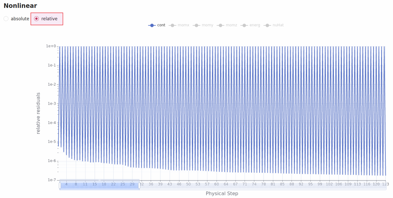
Fig. 7.6.7 Example of unsteady residuals showing at least two orders of magnitude drop within each physical step.#
Starting from an initial solution#
Initializing an unsteady simulation with a well-developed flow field is recommended. A steady-state simulation or a first-order (i.e., orderOfAccuracy: 1) unsteady simulation with few physical steps are often effective to initialize the flow field. The intended second-order (i.e., orderOfAccuracy: 2) unsteady simulation can be forked from the initialization case.
More information about first and second order simulations can be found in Navier-Stokes solver.
Checking the user log#
The next step is to check the flow360_case.user.log file. When a case is running for at least some physical steps and then diverges, reducing the initial value for the CFL number can help to avoid divergence. Often it happens that for an unsteady simulation with a mesh that has a very small initial height in the boundary layer, an initial CFL value of less than 1 can help to avoid divergence. In that case, ramping the CFL value can be used to avoid lengthy iterations to achieve at least two order of magnitude residual drop in a physical step.
Reducing the time-step size#
The time-step size can also be reduced to help address the divergence issue. The time-step size can be set properly for an unsteady simulation based on the minimum edge-length in the mesh and the CFL number. It also can be set based on the Strouhal number and how a physical phenomena is changing with time. Specifying a time-step size that relates to 100-200 steps per flow phenomena (e.g., vortex shedding frequency) is often appropriate.
Reducing the final value of CFL number#
If an unsteady simulation starts, and the time-step size is properly chosen, the final value of the CFL number can be reduced to address the divergence issue.
Increasing the ramp step#
If an unsteady simulation starts, the time-step size is properly chosen, and the final value of the CFL number doesn’t cause divergence, the ramp steps and corresponding number of pseudo-steps can be increased to address the divergence issue.
Final Considerations#
Checking the maximum residual#
For both unsteady and steady simulations, in the event that the above mentioned recommendations did not help to address the divergence, analyzing the residuals in the flow field may be required. Residual data can be included in volumetric solution outputs and postprocessed. See entries starting with residual in the Solver Configuration Output section.
Sudden divergence without proper cause#
If none of the above issues could address the divergence issue please contact the Flexcompute support team (support@flexcompute.com) and let us help you with your simulation.