Non-Dimensional Outputs

Note

With User Variables, manual dimensionalization is rarely needed — simply request the desired unit system and the conversion is automatic. The formulas below describe the underlying logic.

All solver outputs are non-dimensional. To recover physical (SI) values, multiply by the appropriate reference quantity from the Reference Quantities Table.

Reference values for non-dimensional outputs

Property	Ref. value for nondim.	Examples of non-dimensional outputs in Flow360
Length	\(L_\text{gridUnit}\)	wallDistance
Density	\(\rho_\infty\)	primitiveVars
Velocity	\(U_\text{scale}\) (reference velocity scaling)	primitiveVars
Pressure	\(\rho_\infty U_\text{scale}^2\) where \(U_\text{scale}\) is the reference velocity scaling	primitiveVars, nodeForcesPerUnitArea
Pressure Time Derivative	\(\rho_\infty U_\text{scale}^3 / L_\text{gridUnit}\) where \(U_\text{scale}\) is the reference velocity scaling	pressureTimeDerivative
Temperature	\(T_\infty\)	T
Heat Flux	\(\rho_\infty U_\text{scale}^3\) where \(U_\text{scale}\) is the reference velocity scaling	heatFlux
BET, Actuator Disk and Porous Media Force	\(\rho_\infty U_\text{scale}^2 L_\text{gridUnit}^2\) where \(U_\text{scale}\) is the reference velocity scaling	force in BET output
BET, Actuator Disk and Porous Media Moment	\(\rho_\infty U_\text{scale}^2 L_\text{gridUnit}^3\) where \(U_\text{scale}\) is the reference velocity scaling	moment in BET output

Note

Many output variables use the reference velocity scaling \(U_\text{scale}\) (not \(U_\text{ref}\)). In the examples below we assume \(U_\text{scale}\) has been computed as shown in the Introduction.

Visualization Field Conversions

Flow360 exports ParaView (.pvtu) and Tecplot (.szplt) files. All exported fields are non-dimensional. The subsections below show how to recover dimensional values.

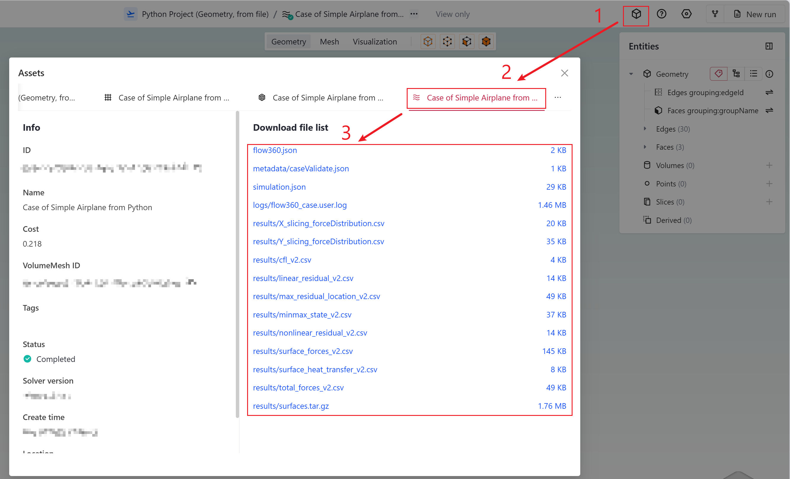
Accessing case results.

Velocity

Reference value: \(U_\text{scale}\).

If velocityX = 0.6 and \(U_\text{scale} = 340\;\text{m/s}\), then \(v_x = 0.6 \times 340 = 204\;\text{m/s}\).

Pressure

Reference value: \(\rho_\infty\,U_\text{scale}^2\).

If p = 0.65, \(\rho_\infty = 1.225\;\text{kg/m}^3\), and \(U_\text{scale} = 340\;\text{m/s}\):

(1)\[p_\text{dim} = 0.65 \times 1.225 \times 340^2 = 92\,046.5\;\text{Pa}\]

Pressure Time Derivative

Reference value: \(\rho_\infty\,U_\text{scale}^3 / L_\text{gridUnit}\), equivalently the pressure reference \(\rho_\infty\,U_\text{scale}^2\) divided by \(L_\text{gridUnit} / U_\text{scale}\). As everywhere else on this page, \(U_\text{scale}\) is the reference velocity scaling, so this one expression covers both gas and liquid operating conditions.

If pressureTimeDerivative = 0.01, \(\rho_\infty = 1.225\;\text{kg/m}^3\), \(U_\text{scale} = 340\;\text{m/s}\), and \(L_\text{gridUnit} = 1\;\text{m}\):

(2)\[\left(\frac{\partial p}{\partial t}\right)_\text{dim} = 0.01 \times \frac{1.225 \times 340^3}{1} = 481\,474\;\text{Pa/s}\]

The same reference applies to pressureTimeDerivative_rms, since a root-mean-square carries the units of the field it is taken over. See Pressure Time Derivative in the output configuration guide for what the field is and how to request it.

Node Force Per Unit Area

nodeForcesPerUnitArea is the total (pressure + friction) force at a node divided by the surface area attributed to that node. Integrating over the whole surface yields the total force. The reference value is the same as for pressure: \(\rho_\infty\,U_\text{scale}^2\).

Temperature

Reference value: \(T_\infty\). Multiply the non-dimensional temperature by the freestream temperature to obtain Kelvin.

Surface Coefficient Definitions

The following coefficients appear in both visualization files and CSV files. They all use the reference velocity \(U_\text{ref}\) (accessed via case.params.reference_velocity), which is different from \(U_\text{scale}\).

Tip

Flow360’s unit system carries SI units through arithmetic, so you can convert any coefficient to physical units in one step. For example, once q_ref and A_ref are retrieved from the API:

tau_wall = (Cf * q_ref).to('Pa')           # wall shear stress
p_dim    = (Cp * q_ref + p_inf).to('Pa')   # static pressure

We define the dynamic pressure for coefficients as:

(3)\[q_\text{ref} = \tfrac{1}{2}\,\rho_\infty\,U_\text{ref}^2\]

Skin Friction Coefficient

The skin friction coefficient vector \(\mathbf{C_f}\) and its magnitude \(C_f\):

(4)\[\mathbf{C_f} = \frac{\mathbf{\tau_\text{wall}}}{q_\text{ref}}\]

To recover the dimensional wall shear stress:

(5)\[\tau_\text{wall}\;[\text{Pa}] = C_f \cdot q_\text{ref}\]

Pressure Coefficient

(6)\[C_p = \frac{p - p_\infty}{q_\text{ref}}\]

To recover the dimensional static pressure:

(7)\[p\;[\text{Pa}] = C_p \cdot q_\text{ref} + p_\infty\]

Total Pressure Coefficient

(8)\[C_{p_t} = \frac{p_t - p_{t,\infty}}{q_\text{ref}}\]

To recover the dimensional total pressure:

(9)\[p_t\;[\text{Pa}] = C_{p_t} \cdot q_\text{ref} + p_{t,\infty}\]

The total pressure coefficient can also be computed from the primitive variables as described in equations 26 and 29 of this paper:

(10)\[C_{p_t} = \frac{\gamma\,p\,\bigl(1 + \tfrac{\gamma-1}{2}\,\text{Ma}^2\bigr)^{\gamma/(\gamma-1)} - \bigl(1 + \tfrac{\gamma-1}{2}\,\text{Ma}_\infty^2\bigr)^{\gamma/(\gamma-1)}}{\tfrac{\gamma}{2}\,\text{Ma}_\infty^2}\]

where \(\gamma = 1.4\) for standard air.

Note

Ensure Mach and primitiveVars are included in your volume output configuration.

CSV File Outputs

Actuator Disk

The file actuatorDisk_output_v2.csv reports power, force, and moment for each disk. The power column contains a coefficient:

(11)\[C_p = \frac{\text{Power}\;[\text{W}]}{\rho_\infty\,U_\text{scale}^3\,L_\text{gridUnit}^2}\]

To obtain dimensional power:

actuator_disk_output = case.results.actuator_disks.averages
density = case.params.operating_condition.thermal_state.density
L_grid  = project.length_unit

C_p   = actuator_disk_output['Disk0_Power']
power = C_p * density * U_scale**3 * L_grid**2      # W

Attention

Actuator Disk forces and moments use \(U_\text{scale}\), not \(U_\text{ref}\). See Converting to Physical Units for the general conversion formulas.

BET Loading

The file bet_forces_v2.csv contains:

1. Integrated forces and moments per disk (Disk0_Force_x, Disk0_Moment_x, …). These are non-dimensional raw values:

   (12)\[\text{Force}^* = \frac{F\;[\text{N}]}{\rho_\infty\,U_\text{scale}^2\,L_\text{gridUnit}^2}\]
   (13)\[\text{Moment}^* = \frac{M\;[\text{N·m}]}{\rho_\infty\,U_\text{scale}^2\,L_\text{gridUnit}^3}\]

   Note

   These values represent forces/moments on the solid. Forces on the fluid are the negative of the above.

   Note

   Equations Eq.(12) and Eq.(13) also apply to Porous Media outputs in porous_media_output_v2.csv.

   Attention

   BET forces and moments use \(U_\text{scale}\), not \(U_\text{ref}\). The x, y, z components are in the global inertial frame defined by the mesh.

2. Sectional thrust \(C_t\) and torque \(C_q\) per blade at each radial station (Disk0_Blade0_R0_ThrustCoeff, …).

   (14)\[C_t(r) = \frac{\text{Thrust/span}\;[\text{N/m}]}{\tfrac{1}{2}\,\rho_\infty\,(\Omega r)^2\,\text{chord}_\text{ref}} \cdot \frac{r}{R}\]
   (15)\[C_q(r) = \frac{\text{Torque/span}\;[\text{N}]}{\tfrac{1}{2}\,\rho_\infty\,(\Omega r)^2\,\text{chord}_\text{ref}\,R} \cdot \frac{r}{R}\]

   Here \(r\) is the dimensional distance from the rotation axis, \(\text{chord}_\text{ref}\) the dimensional reference chord, and \(R\) the rotor radius.

   Note

   \(C_t\) and \(C_q\) are sectional loadings: \(C_t(r) = \text{d}C_T/\text{d}(r/R)\) and \(C_q(r) = \text{d}C_Q/\text{d}(r/R)\).

   Important

   All right-hand-side quantities in Eq.(12)–Eq.(15) are dimensional. The non-dimensional radius in the CSV must first be converted: \(r\) = Disk0_Blade0_R0_Radius \(\times\, L_\text{gridUnit}\).

   Warning

   For steady-state BET Disk simulations, \(C_t\) and \(C_q\) are written only for Blade0; all other blades report zeros because the loading is identical. For unsteady BET Line simulations each blade has distinct values.

Python example — dimensional force, moment, and sectional loading:

bet_forces = case.results.bet_forces.averages
density    = case.params.operating_condition.thermal_state.density
L_grid     = project.length_unit

# --- Integrated force & moment (Disk 0) ---
force_x  = bet_forces["Disk0_Force_x"]  * density * U_scale**2 * L_grid**2     # N
moment_x = bet_forces["Disk0_Moment_x"] * density * U_scale**2 * L_grid**3     # N·m

# --- Sectional loading (Disk 0, Blade 0, radial station 1) ---
bet_model  = case.params.models[4]   # index of the BETDisk model
chord_ref  = bet_model.chord_ref
omega      = bet_model.omega
R          = bet_model.entities.stored_entities[0].outer_radius

r1    = bet_forces["Disk0_Blade0_R1_Radius"]
Ct_r1 = bet_forces["Disk0_Blade0_R1_ThrustCoeff"]
Cq_r1 = bet_forces["Disk0_Blade0_R1_TorqueCoeff"]

thrust_r1 = Ct_r1 * 0.5 * density * omega**2 * r1 * L_grid * R * chord_ref     # N/m
torque_r1 = Cq_r1 * 0.5 * density * omega**2 * r1 * L_grid * R**2 * chord_ref  # N

Aeroacoustic Output

The file total_acoustics_v3.csv reports the non-dimensional acoustic pressure signal at each observer location. If AeroacousticOutput.write_per_surface_output is True, per-surface files surface_<name>_acoustics_v3.csv are also written.

Columns: time, physical_step, observer_0_pressure, observer_0_thickness, observer_0_loading, … for N+1 observers.

Note

The observation time may fall outside the simulation time range because the acoustic signal takes a finite propagation time from the surface to each observer. Early and late time entries are zero-padded.

Heat Transfer

The file surface_heat_transfer_v2.csv contains surface-integrated heat flux in non-dimensional form.

To recover the dimensional heat transfer rate, multiply by \(\rho_\infty\,U_\text{scale}^3\,L_\text{gridUnit}^2\):

surface_ht = case.results.surface_heat_transfer.averages
density    = case.params.operating_condition.thermal_state.density
L_grid     = project.length_unit

q_nd = surface_ht["fluid/Interface_solid_HeatTransferRate"]
q    = q_nd * density * U_scale**3 * L_grid**2   # W

Visualization Tips

The sections below are not about conversion formulas but about using specific output fields effectively.

Skin Friction — Detecting Separation

The CfVec vector is useful for locating boundary-layer separation. Fully attached flow follows the surface along the streamwise direction; separated flow produces local recirculation with reversed skin friction.

For flow predominantly in the x-direction, regions of negative CfVecX indicate separation. Visualizing with a three-level scale (e.g. −1e-6, 0, 1e-6) highlights separated vs. attached regions:

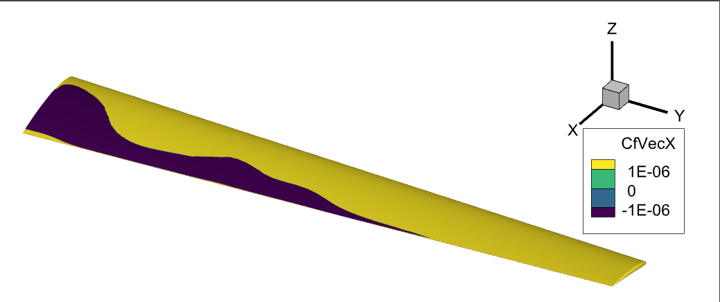
x-component of skin friction showing attached (yellow) and separated (purple) flow at high angle of attack.

Surface streamlines can also reveal recirculation. Since wall velocity is zero on a NoSlipWall, use CfVec{X,Y,Z} as the integration variable instead of velocity:

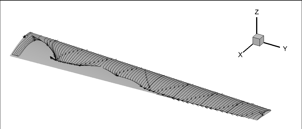
Surface streamlines showing recirculation regions.

Total Pressure — Visualizing Separation and Boundary Layers

\(C_{p_t}\) reveals separation regions in volume slices and is effective for visualizing the boundary layer:

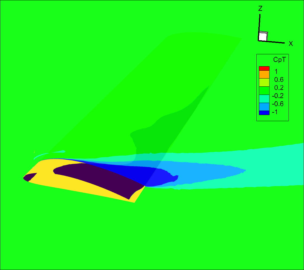
Total pressure coefficient on a slice through a partially stalled wing.

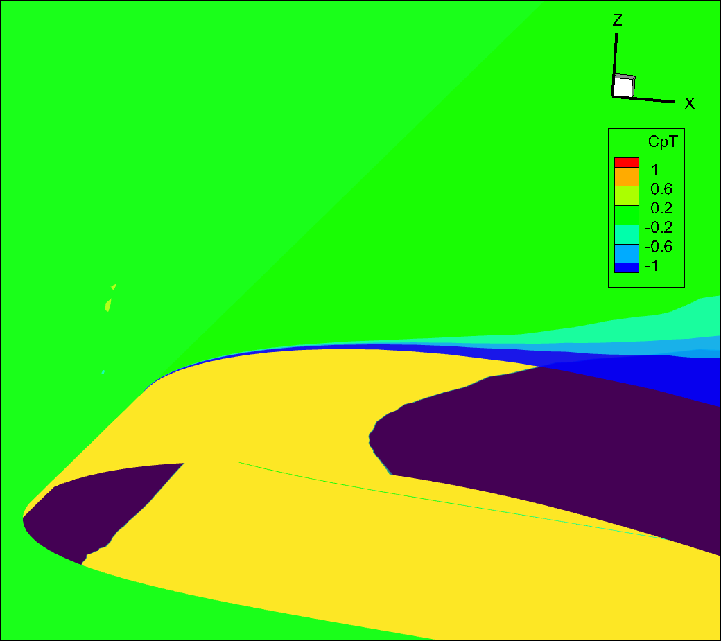
Zoomed view showing the developing boundary layer (blue) near the leading edge.

Q-Criterion — Visualizing Vortices

The qcriterion field identifies vortices via isosurfaces. Recommended isosurface values:

• Aircraft: \(\text{Ma}^2 / \text{span}^2\)

• Rotors: \(\text{Ma}_\text{tip}^2 / D^2\)

Larger values show only strong vortices; smaller values reveal weaker structures.

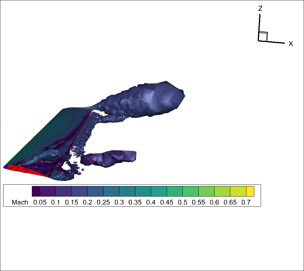
qcriterion isosurface showing tip vortex and vortices from the separation region.

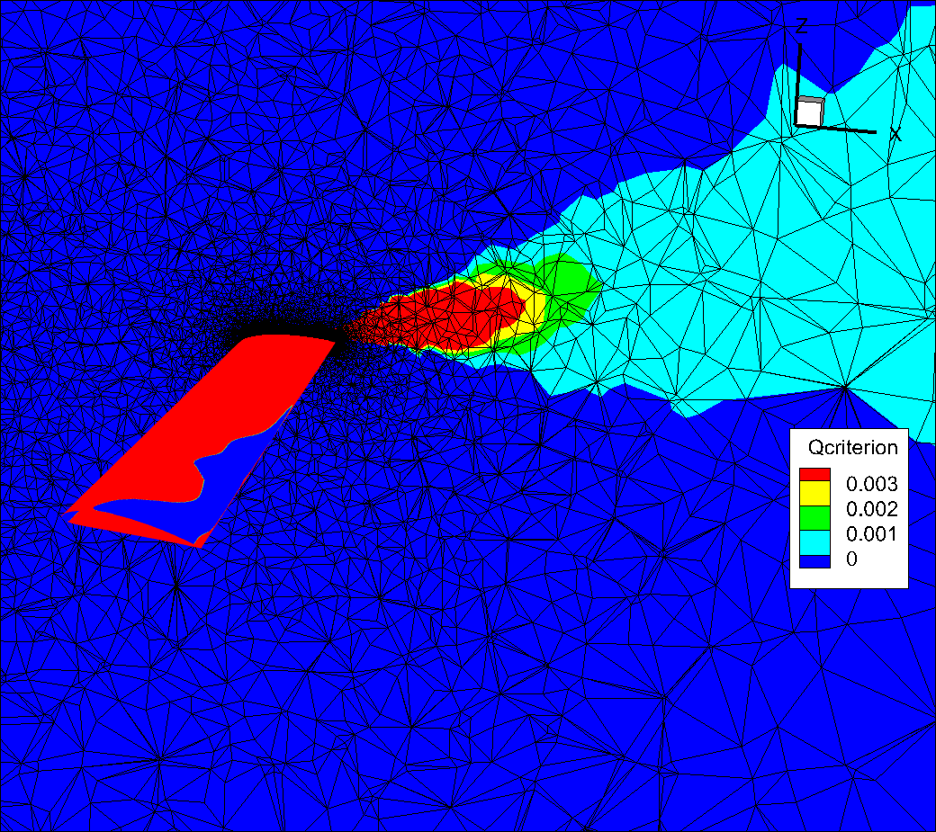
Volume mesh coarsening away from the wing causes rapid vortex dissipation.

After refining the far-field mesh:

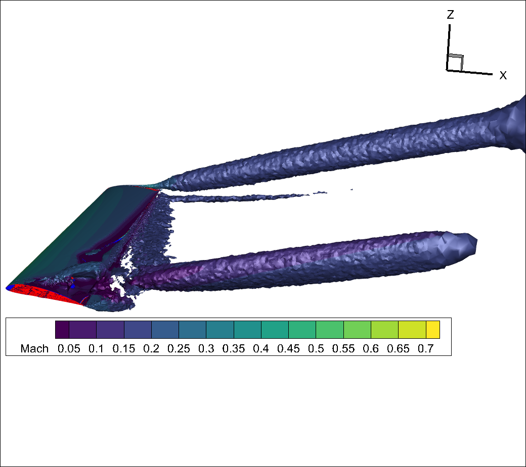
Smoother isosurface with improved vortex resolution on a refined mesh.

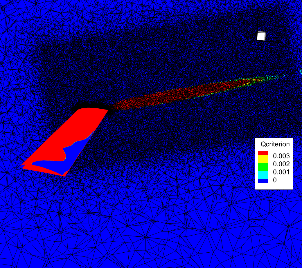
Refined volume mesh reduces numerical dissipation.

For more Q-criterion visualizations:

• BET Line flow visualization

• Wind turbine case study

• Hover prediction workshop (figs 9, 17)

• Rotor modeling techniques (figs 11, 12, 26, 27)

• Rotor5 tool (figs 4, 18, 19)

• XV15 DES simulations (figs 10, 14, 17)