
Hinge Torques Monitoring#
Note: The settings in this example are by no means a validation setup; they are crafted to showcase the capabilities of Flow360 and we have intentionally reduced node count and example FC cost. For rigorous validation, modify the settings as needed.
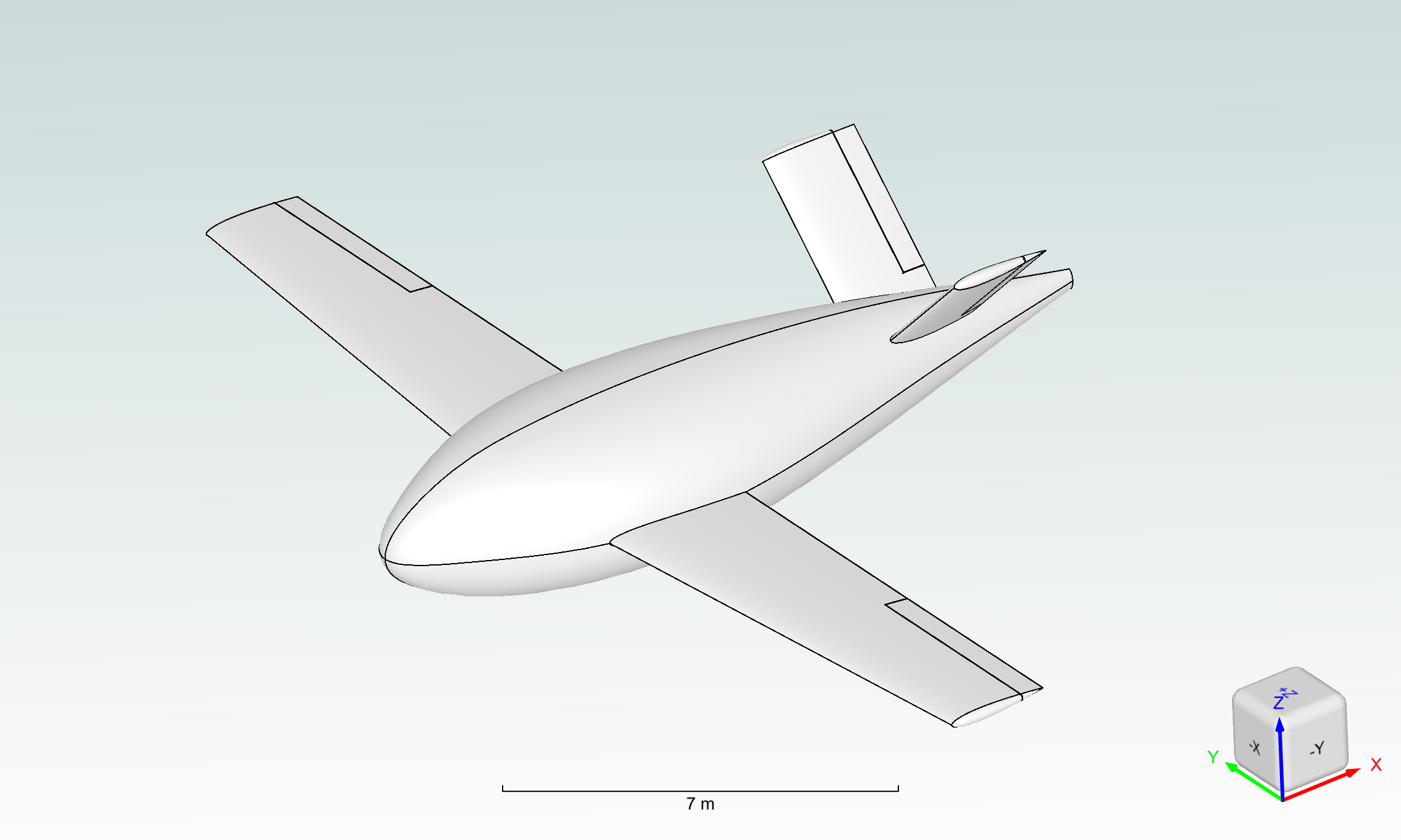
This tutorial will show how to set up a case where moments on specific surfaces are monitored throughout the simulation. The content will cover:
creating a project from a geometry,
meshing using the beta mesher and automated farfield,
setup of a steady case,
setup of
SurfaceIntegralOutputusingUserVariableto capture hinge moments on control surfaces,results postprocessing.
1. Imports and Project Creation#
To begin working with the Flow360 API it is necessary to firstly import the flow360 python package that will be the interface between you and the software. The files necessary for this example are being downloaded through the TutorialUDDForcesMoments example.
All simulations are managed through the Project object, which stores all the runs associated with a certain root asset. Root asset can be a geometry, surface mesh or volume mesh. In case of this tutorial the Project will be started from the geometry.
[1]:
import flow360 as fl
from flow360.examples import TutorialUDDForcesMoments
[2]:
TutorialUDDForcesMoments.get_files()

project = fl.Project.from_geometry(
    TutorialUDDForcesMoments.geometry, name="Hinge Torques Monitoring"
)
[12:17:22] INFO: The file (UDD_FM_airplane.csm) is being downloaded, please
           wait.
           WARNING: DeprecationWarning: `length_unit` was not specified and
           defaults to 'm'. Relying on this default is deprecated and will be
           removed in a future release; specify the length unit of your
           geometry/mesh explicitly to avoid silent unit/scale mistakes.
[12:17:39] INFO: Geometry successfully submitted:
                   type        = Geometry
                   name        = Hinge Torques Monitoring
                   id          = geo-3996703c-31fc-42d1-a886-8afca1f752de
                   status      = uploaded
                   project id  = prj-cd69ce66-3cf6-450c-b31e-d9c62cb0f2a2

           INFO: Waiting for geometry to be processed.
If the Project has already been created before it is possible to retrieve it using its unique ID.
[3]:
# project=fl.Project.from_cloud("prj-e8aa4e7a-a6b8-47f5-97c4-7e64bbf76aeb")
Project contains all the information about its root asset, in this case - geometry. To be able to correctly reference it it is necessary to group the faces and edges by the attribute that was assigned to distinguish the faces in a CAD file.
[4]:
geometry = project.geometry

geometry.group_edges_by_tag("edgeName")
geometry.group_faces_by_tag("groupName")

print("Geometry boundaries:")
for boundary in geometry.entity_info.get_boundaries():
    print(f"- {boundary.name}")
[12:18:12] INFO: Regrouping face entities under `groupName` tag (previous
           `faceId`).
Geometry boundaries:
- fuselage
- wingRight
- wingLeft
- vTailRight
- vTailLeft
- rudderLeft
- rudderRight
- aileronLeft
- aileronRight
2. Meshing#
When the projects starts from the geometry it is necessary to set up the automated meshing workflow.
Firstly the AutomatedFarfield object is created to indicate that the geometry only contains the simulated object and the farfield has to be created around it.
Then the defaults for meshing are defined. Those are the “global” settings for the mesher.
[5]:
farfield = fl.AutomatedFarfield()

with fl.SI_unit_system:
    meshing = fl.MeshingParams(
        defaults=fl.MeshingDefaults(
            surface_max_edge_length=0.5,
            curvature_resolution_angle=10 * fl.u.deg,
            boundary_layer_first_layer_thickness=2e-6,
            boundary_layer_growth_rate=1.2,
        ),
        volume_zones=[farfield],
    )
INFO: using: SI unit system for unit inference.
To refine specific parts of the mesh the refinements field is used, where user can define surface (such as SurfaceRefinement and SurfaceEdgeRefinement) and volumetric refinements (UniformRefinement).
It is worth to notice how the specific parts of the geometry are referenced using the geometry object. They can be then referenced using face names directly or through a wildcard entry (*).
[6]:
with fl.SI_unit_system:
    box1 = fl.Box(name="box1", size=[2, 6, 3], center=[6.5, 9, 0], axis_of_rotation=[0, 1, 0])
    box2 = fl.Box(name="box2", size=[2, 6, 3], center=[6.5, -9, 0], axis_of_rotation=[0, 1, 0])
    box3 = fl.Box(name="box3", size=[4, 8, 3], center=[12, 0, 2], axis_of_rotation=[0, 1, 0])

    meshing.refinements.extend(
        [
            fl.SurfaceEdgeRefinement(
                method=fl.AngleBasedRefinement(value=1 * fl.u.deg),
                edges=[geometry["leadingEdge"]],
            ),
            fl.SurfaceEdgeRefinement(
                method=fl.HeightBasedRefinement(value=5e-3),
                edges=[geometry["trailingEdge"]],
            ),
            fl.SurfaceRefinement(max_edge_length=0.5, faces=[geometry["wing*"]]),
            fl.UniformRefinement(name="box_refinement1", entities=[box1, box2, box3], spacing=0.2),
        ]
    )
INFO: using: SI unit system for unit inference.
3. Boundary Conditions, Flow physics and numerics settings#
To describe the physical behaviour of the flow the Boundary Conditions or surface models are used. In this case the ones needed would be the Freestream condition that is assigned to the farfield and the Wall condition for the object. The Fluid model is a volume model that enables access to the controls of the fluid solver.
The operating_condition is responsible for defining the fluid behaviour at the freestream and is used to set the velocity, angle of attack and the thermal state of the fluid in this case.
reference_geometry defines values that are used as a reference when calculating various coefficients.
Finally time_stepping describes whether the simulation is steady or transient and how many time (or pseudo time) steps should be performed.
[7]:
with fl.SI_unit_system:
    reference_geometry = fl.ReferenceGeometry(
        area=60, moment_center=[5.7542, 0, 0], moment_length=[1, 1, 1]
    )
    operating_condition = fl.AerospaceCondition(
        velocity_magnitude=50,
        alpha=10 * fl.u.deg,
        atmosphere=fl.ThermalState(temperature=288.15),
    )
    models = [
        fl.Fluid(
            navier_stokes_solver=fl.NavierStokesSolver(
                absolute_tolerance=1e-9,
                linear_solver=fl.LinearSolver(max_iterations=35),
            ),
            turbulence_model_solver=fl.SpalartAllmaras(
                linear_solver=fl.LinearSolver(max_iterations=25)
            ),
        ),
        fl.Wall(
            surfaces=[geometry["*Left"], geometry["*Right"], geometry["fuselage"]],
        ),
        fl.Freestream(surfaces=[farfield.farfield]),
    ]
    time_stepping = fl.Steady(max_steps=5000)
[12:18:13] INFO: using: SI unit system for unit inference.
4. Definition of UserVariables#
In the next cell, we define several custom UserVariables to compute hinge torques for the control surfaces (right/left ailerons and right/left rudders). Each variable calculates the local contribution to the hinge torque by taking the moment (cross product) of the force per unit area about a specified torque center, and then projecting that moment onto the relevant hinge axis. The resulting user variables represent the hinge torque per unit area at each surface node, with units of pressure
times length (Pa·m), and can be integrated over the relevant surfaces to obtain the total hinge torque values.
Note: The variables are defined per unit area because
SurfaceIntegralOutputintegrates over the surface area, not over individual nodes.
[8]:
right_aileron_torque_center = [5.7542, 7, 0] * fl.u.m
right_aileron_torque_axis = [0, 1, 0]

right_aileron_hinge_torque_partial_dim = fl.UserVariable(
    name="right_aileron_hinge_torque_partial",
    value=fl.math.dot(
        fl.math.cross(
            fl.math.subtract(fl.solution.coordinate, right_aileron_torque_center),
            fl.solution.node_forces_per_unit_area,
        ),
        right_aileron_torque_axis,
    ),
).in_units(new_unit=fl.u.Pa * fl.u.m)

left_aileron_torque_center = [5.7542, -7, 0] * fl.u.m
left_aileron_torque_axis = [0, -1, 0]

left_aileron_hinge_torque_partial_dim = fl.UserVariable(
    name="left_aileron_hinge_torque_partial",
    value=fl.math.dot(
        fl.math.cross(
            fl.math.subtract(fl.solution.coordinate, left_aileron_torque_center),
            fl.solution.node_forces_per_unit_area,
        ),
        left_aileron_torque_axis,
    ),
).in_units(new_unit=fl.u.Pa * fl.u.m)

right_rudder_torque_center = [12.01, 0.861, 0.861] * fl.u.m
right_rudder_torque_axis = [0, fl.math.sqrt(2) / 2, fl.math.sqrt(2) / 2]

right_rudder_hinge_torque_partial_dim = fl.UserVariable(
    name="right_rudder_hinge_torque_partial",
    value=fl.math.dot(
        fl.math.cross(
            fl.math.subtract(fl.solution.coordinate, right_rudder_torque_center),
            fl.solution.node_forces_per_unit_area,
        ),
        right_rudder_torque_axis,
    ),
).in_units(new_unit=fl.u.Pa * fl.u.m)

left_rudder_torque_center = [12.01, -0.861, 0.861] * fl.u.m
left_rudder_torque_axis = [0, -fl.math.sqrt(2) / 2, fl.math.sqrt(2) / 2]

left_rudder_hinge_torque_partial_dim = fl.UserVariable(
    name="left_rudder_hinge_torque_partial",
    value=fl.math.dot(
        fl.math.cross(
            fl.math.subtract(fl.solution.coordinate, left_rudder_torque_center),
            fl.solution.node_forces_per_unit_area,
        ),
        left_rudder_torque_axis,
    ),
).in_units(new_unit=fl.u.Pa * fl.u.m)
Below, each hinge torque user variable (representing the torque per unit area contribution) is integrated over the corresponding control surface using SurfaceIntegralOutput. These integrals compute the total hinge torque for each control surface (right/left aileron and rudder) by summing their local torque contributions defined above.
The output_fields for each surface integral specify which user variable is integrated, and the surfaces parameter specifies which part of the geometry the integration is applied to.
[9]:
outputs = [
    fl.SurfaceIntegralOutput(
        name="right_aileron_hinge_torque",
        output_fields=[right_aileron_hinge_torque_partial_dim],
        surfaces=geometry["aileronRight"],
    ),
    fl.SurfaceIntegralOutput(
        name="left_aileron_hinge_torque",
        output_fields=[left_aileron_hinge_torque_partial_dim],
        surfaces=geometry["aileronLeft"],
    ),
    fl.SurfaceIntegralOutput(
        name="right_rudder_hinge_torque",
        output_fields=[right_rudder_hinge_torque_partial_dim],
        surfaces=geometry["rudderRight"],
    ),
    fl.SurfaceIntegralOutput(
        name="left_rudder_hinge_torque",
        output_fields=[left_rudder_hinge_torque_partial_dim],
        surfaces=geometry["rudderLeft"],
    ),
]
5. SimulationParams#
Finally all of the previously defined fields are input to the SimulationParams object that defines a whole process from meshing to performing the simulation.
After preparing those parameters the simulation can be kicked off using the run_case command.
[10]:
with fl.SI_unit_system:
    params = fl.SimulationParams(
        meshing=meshing,
        operating_condition=operating_condition,
        reference_geometry=reference_geometry,
        models=models,
        outputs=outputs,
    )

case = project.run_case(params, name="Steady RANS (hinge moments)", use_beta_mesher=True)
           INFO: using: SI unit system for unit inference.

[12:18:14] WARNING: The spacing of 0.2 m specified in UniformRefinement will be
           cast to the first lower refinement in the octree series (0.125 m).
           INFO:
           INFO: Units of output `UserVariables`:
           INFO:
           ------------------------------------------------------------------
           INFO: Variable Name                                         | Unit
           INFO:
           ------------------------------------------------------------------
           INFO: left_aileron_hinge_torque_partial                     | Pa*m
           INFO: left_rudder_hinge_torque_partial                      | Pa*m
           INFO: right_aileron_hinge_torque_partial                    | Pa*m
           INFO: right_rudder_hinge_torque_partial                     | Pa*m
           INFO: right_aileron_hinge_torque_partial (Surface integral) | Pa*m**3
           INFO: left_aileron_hinge_torque_partial (Surface integral)  | Pa*m**3
           INFO: right_rudder_hinge_torque_partial (Surface integral)  | Pa*m**3
           INFO: left_rudder_hinge_torque_partial (Surface integral)   | Pa*m**3
           INFO:
           ------------------------------------------------------------------
           INFO:
[12:18:15] INFO: Selecting beta/in-house mesher for possible meshing tasks.
[12:18:17] INFO: Successfully submitted:
                   type        = Case
                   name        = Steady RANS (hinge moments)
                   id          = case-f2d73218-b5e9-480f-b082-3507ba7974ad
                   status      = pending
                   project id  = prj-cd69ce66-3cf6-450c-b31e-d9c62cb0f2a2
6. Accessing the results#
The case.wait() command waits for the simulation to be finished before it is possible to access its results. After completing the whole set of results can be accessed using the results parameter of case.
[11]:
case.wait()
results = case.results
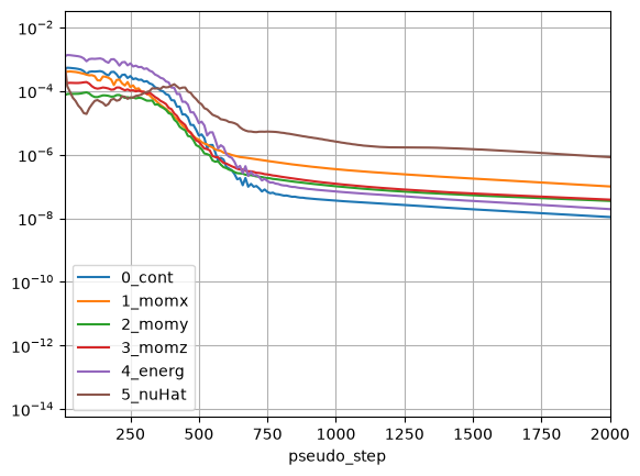
The cell below shows how to quickly view the convergence of a simulation, but other results are available such as:
forces
monitors
aeroacoustics results
user defined dynamics monitoring
and others
[12]:
nonlinear_residuals_data = results.nonlinear_residuals.as_dataframe()
nonlinear_residuals_data.plot(
    "pseudo_step",
    ["0_cont", "1_momx", "2_momy", "3_momz", "4_energ", "5_nuHat"],
    logy=True,
    xlim=[10, 2000],
    grid=True,
)
[12:38:41] INFO: Saved to
           /tmp/tmph6i7tr3b/9071ce30-a06d-4afb-a07a-de4274232967.csv
[12]:
<Axes: xlabel='pseudo_step'>
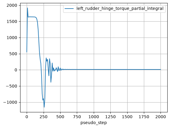
To access the hinge torque history that was set with the SurfaceIntegralOutput, the monitors result type should be accessed.
[13]:
left_rudder_hinge_torque_history = results.monitors["left_rudder_hinge_torque"].as_dataframe()
left_rudder_hinge_torque_history.plot(
    "pseudo_step", "left_rudder_hinge_torque_partial_integral", grid=True
)
[12:38:43] INFO: Saved to
           /tmp/tmph6i7tr3b/55d48688-231d-4de1-9805-e2b448308a5d.csv
[13]:
<Axes: xlabel='pseudo_step'>