Points

Points#

A comprehensive guide to monitoring and analyzing flow properties at specific locations in the simulation domain using Points and Point Arrays.

Available Creation Methods#

Type	Description
Point	Single monitoring location in 3D space
Point array	Multiple monitoring points along a straight line defined by its start and end points
2D point array	Points on a two-dimensional grid
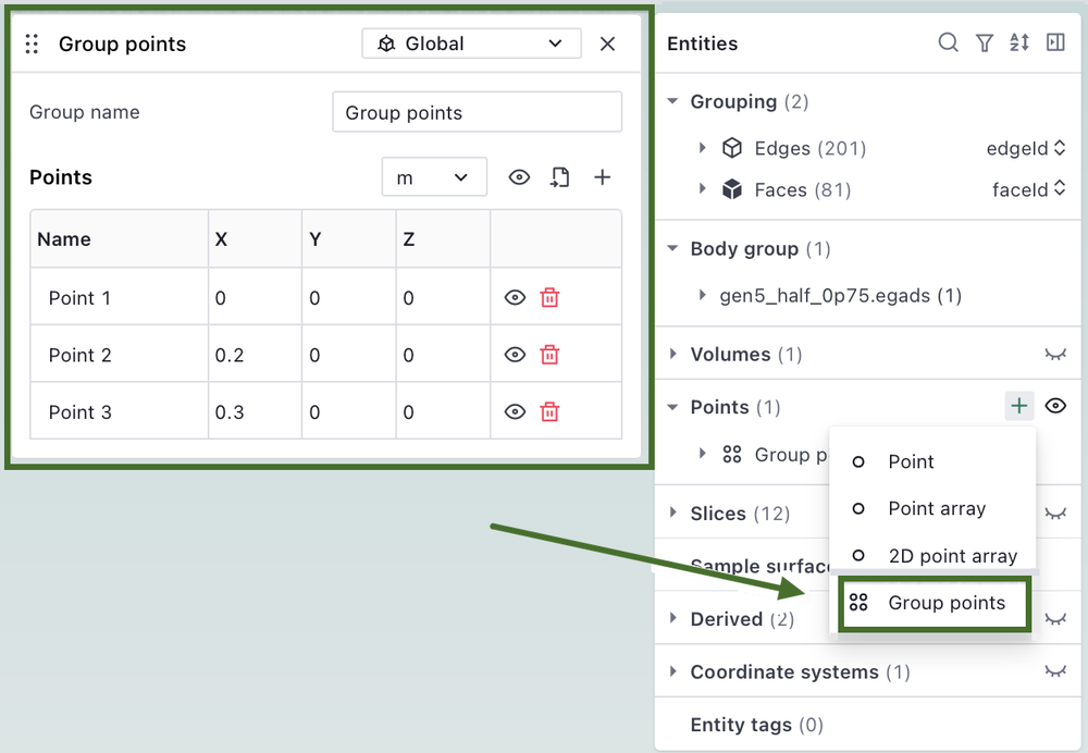
Group points	A named group of explicitly listed points, typed in or imported from a CSV file

Detailed Descriptions#

Point#

Defines a single monitoring location in three-dimensional space for tracking flow properties.

Point Parameters:

Position: Three-dimensional coordinates (x, y, z)

Point array#

Creates an array of equally spaced points between start and end locations.

Point array Parameters:

Start Position: Three-dimensional coordinates (x, y, z)
End Position: Three-dimensional coordinates (x, y, z)
Number of Points: Integer > 2

Group points#

Groups any number of explicitly listed points under one name.

Create it with the + button of the Points group, which lists Group points after the other point types.

Group points Parameters:

Group name: Name of the group
Coordinate system: Coordinate system of the point coordinates (Global by default), chosen from the menu at the top of the panel
Points: Table of points, each with a name and x, y, z coordinates. Add rows with the + button or import them from a CSV file with the import icon. The eye icon shows the points in the viewer.
Unit: Length unit of the coordinates

The Python equivalent is PointGroup, with PointGroup.from_csv for CSV files.

GroupPoints

Min/max locations#

Shows where the solver variables reached their extreme values, to help find the origin of a divergence.

For a diverged case, the Points group lists Min/max locations. Its panel shows the minimum or maximum value and location of each tracked variable (for example min_rho, min_p, max_umag, min_nuHat, max_nuHat), with a pseudo-step slider to step through the history. The eye icon next to each variable shows its location in the viewer, which works in the Geometry, Mesh and Visualization tabs.

Output Data#

Points and Point arrays provide access to flow field variables at their specified locations, allowing for detailed monitoring and analysis of local flow properties throughout the simulation.

Pressure
Temperature
Velocity components
Density
Turbulence quantities
Vorticity
Other solver-specific variables

Note

To monitor variables at points during a simulation, see Probe Outputs.

❓ Frequently Asked Questions

Can points be placed outside the computational domain?

No, points must be positioned within the computational domain to provide valid results.

🐍 Python Example Usage

import flow360 as fl

# Create a single point at the leading edge
leading_edge_point = fl.Point(
    name="leading_edge",
    location=(1.0, 0.5, 0.0) * fl.u.m
)

# Create a point array for wake analysis
wake_profile = fl.PointArray(
    name="wake_profile",
    start=(0, 0, 0) * fl.u.m,
    end=(5, 0, 0) * fl.u.m,
    number_of_points=10
)

# Group many explicitly listed points under one name
rake = fl.PointGroup(
    name="rake_a",
    locations=[[0.0, 0.0, 0.0], [0.0, 0.0, 1.0]] * fl.u.m,
)

# Or read the coordinates from a CSV file, giving the unit and the x, y, z column names
probes = fl.PointGroup.from_csv(
    "probes.csv",
    name="rake_b",
    unit=fl.u.mm,
    coordinate_columns=("x_coord", "y_coord", "z_coord"),
)

PointGroup.from_csv reads a headerless file of exactly three columns when coordinate_columns is omitted, and drops repeated coordinates with a warning. A point group can be used in probe, surface probe and streamline outputs.