Calculating Dynamic Derivatives using Sliding Interfaces

Calculating Dynamic Derivatives using Sliding Interfaces#

This tutorial demonstrates how to obtain dynamic stability derivatives by oscillating a wing enclosed in a sliding interface.

Geometry and Mesh#

In this example, the geometry is a wing with NACA0012 airfoil. The chord $c$ = 1 m and the span $b$ = 2 m. So the momentLength = [ $b$ /2, $c$ , $b$ /2] = [1, 1, 1]. The momentCenter is set at [0, 0, 0], which is the airfoil quarter-chord point and midspan of the wing. As shown in the following figure, there is a cylindrical sliding interface enclosing the wing. The radius of the cylinder is 1 m and the length is 2.5 m. The rotational center is also located at [0, 0, 0] and the axis of rotation is along the y-axis.

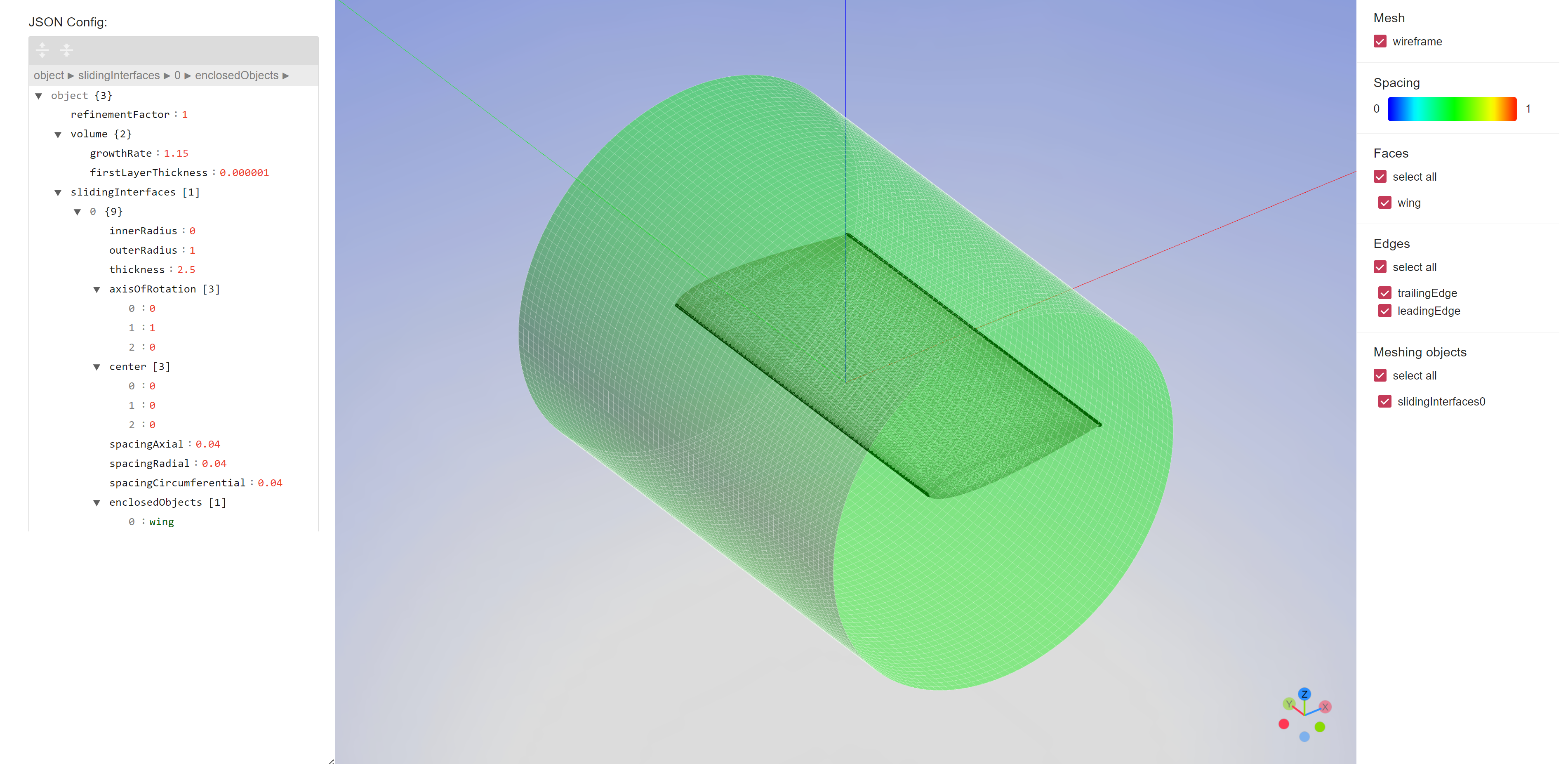
../../_images/wing_in_sliding_interface.png — Fig. 227 Wing enclosed in sliding interface#

The mesh was generated using the automated meshing workflow. The geometry file, surfaceMesh.json and volumeMesh.json are provided so the readers can easily generate the mesh in their account. For more information about this automated meshing workflow please see Automated Meshing.

Case Setup#

The entire simulation contains two cases:

Steady case with a fixed sliding interface for initializing the flow field.
Unsteady case with an oscillating sliding interface for collecting the data.

The steady case is quite trivial since the sliding interface is stationary. For readers’ convenience, the Flow360Steady.json is provided. As for the unsteady case, when preparing the Flow360Unsteady.json, the key is to correctly set up the thetaDegrees input expression:

(23)#

thetaDegrees = A * \sin (omega * t)

Where $A$ is the amplitude of oscillation in degrees, omega is the nondimensional angular frequency of the oscillation, and t is the nondimensional time. Note that omega and t are nondimensional variables of the Flow360 solver.

In this case we set $A = 2$ °, so the pitching angle of the wing is oscillating between $\pm 2$ °. omega is typically computed from the number of flowthroughs per radian, denoted by $n$ . In this example, we have $n = 2.5$ flowthru/rad, which means when omega*t changes 1 radian, the air will flow through 2.5 chord lengths. In this tutorial, the freestream velocity $U_{\infty} = 50$ m/s. The physical angular frequency is given by,

(24)#

ω = \frac{U_{\infty}}{n \cdot c} = \frac{50 m/s}{2.5 \times 1 m} = 20 rad/s

Since we have the freestream speed of sound $C_{\infty} = 340.294$ m/s and gridUnit = 1 m. The nondimensional angular frequency can be written as,

(25)#

omega = \frac{ω}{C_{\infty} / L_{gridUnit}} \approx 0.05877271

Therefore, the slidingInterfaces section is:

"slidingInterfaces": [
    {
        "stationaryPatches": ["stationaryBlock/slidingInterface-0"],
        "rotatingPatches": ["rotatingBlock-0/slidingInterface-0"],
        "axisOfRotation": [0,1,0],
        "centerOfRotation": [0,0,0],
        "volumeName": "rotatingBlock-0",
        "thetaDegrees": "2.00 * sin(0.05877271 * t)"
    }
]

Another critical value we need to set up carefully is the nondimensional timeStepSize. In this example, each period is spilt into 100 steps, therefore,

(26)#

timeStepSize = 0.01 \cdot \frac{2 π}{omega}

Note that the omega in the above equation is the nondimensional angular frequency.

Submission#

The surface/volume meshes and steady/unsteady cases can be easily submitted via our PythonAPI:

surfaceMeshId  = flow360client.NewSurfaceMeshFromGeometry('path/to/geometry.csm', 'path/to/surfaceMesh.json')
volumeMeshId   = flow360client.NewMeshFromSurface(surfaceMeshId=surfaceMeshId, config='path/to/volumeMesh.json')
steadyCaseId   = flow360client.NewCase(meshId=volumeMeshId, config='path/to/SteadyFlow360.json', caseName='dynamic-derivatives-steady')
unsteadyCaseId = flow360client.NewCase(meshId=volumeMeshId, config='path/to/UnsteadyFlow360.json', caseName='dynamic-derivatives-unsteady', parentId=steadyCaseId)

Postprocessing#

Once the case is completed, the user can download the “total_forces_v2.csv”, where the first column is physical_step. Note that the flowfield was initialized from a steady case, so the nondimensional time can be written as,

(27)#

t = physical_step * timeStepSize

In this example, the angle of attack $α$ is always identical to the pitch angle $θ$ ,

(28)#

α = θ = A * \sin (omega * t)

Therefore, $\dot{α}$ is always identical to the pitch rate $q$ . The $\dot{α}$ at time step i can be obtained by finite differencing $α$ at the i-1 and i+1 time step

(29)#

{\dot{α}}_{i} = \frac{α_{i + 1} - α_{i - 1}}{2 * timeStepSize} \frac{C_{\infty}}{L_{gridUnit}} \frac{c}{U_{\infty}}

Note that the unit of $\dot{α}$ in the equation above is rad/flowthru.

As shown in the following plot, when $α = 0$ , $\dot{α}$ will reach the extrema.

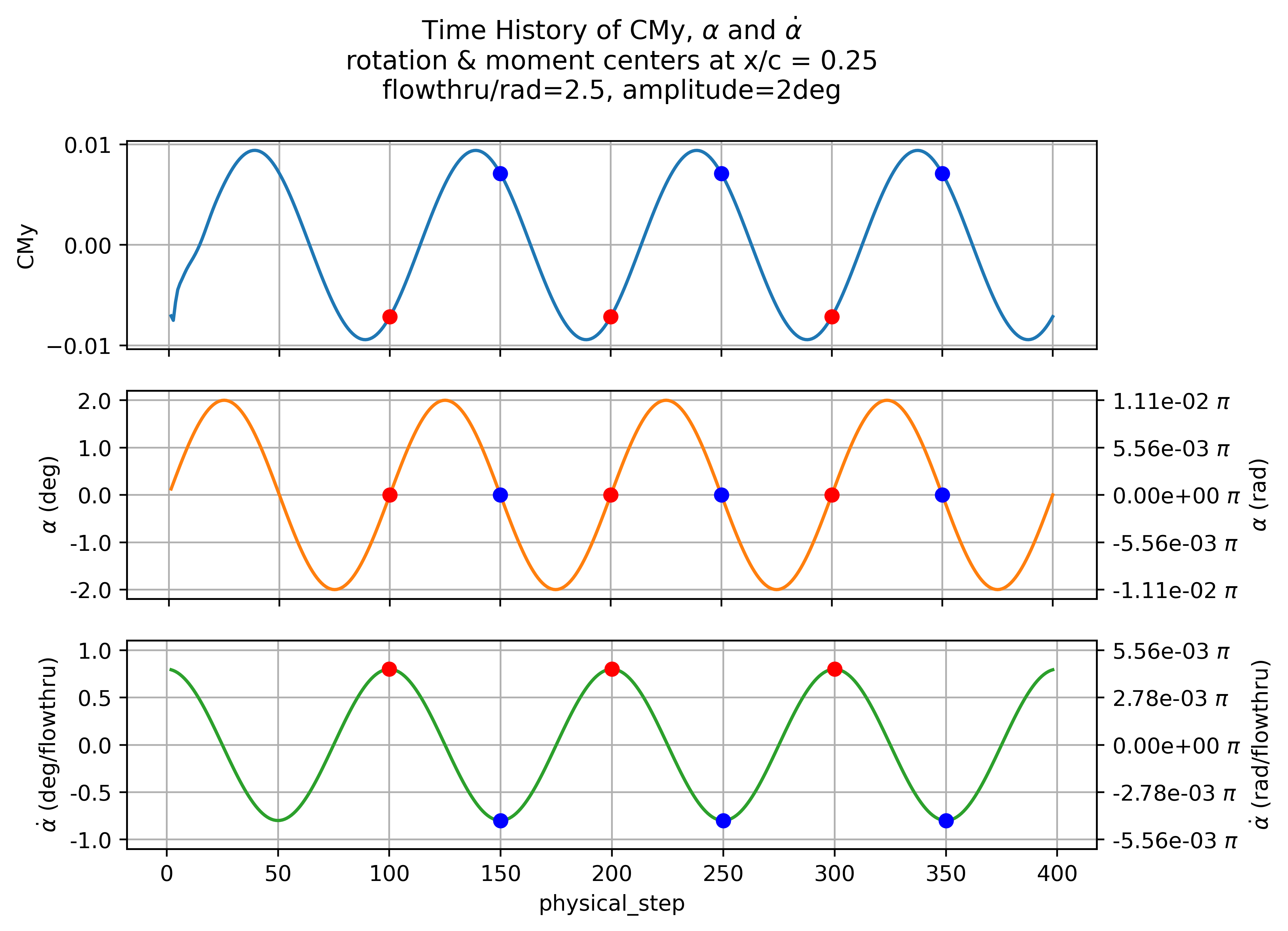
../../_images/timeHistory.png — Fig. 228 Time History of CMy, $α$ and $\dot{α}$ . The blue and red dots show when $\dot{α}$ reaches the extrema.#

If we plot CMy versus $\dot{α}$ and linearly fit the points with $α = 0$ (i.e. min/max $\dot{α}$ ) the slope of the fitted line is the dynamic derivative:

(30)#

\frac{d C M y}{d \dot{α}} = \frac{d C M y}{d q} = - 0.511

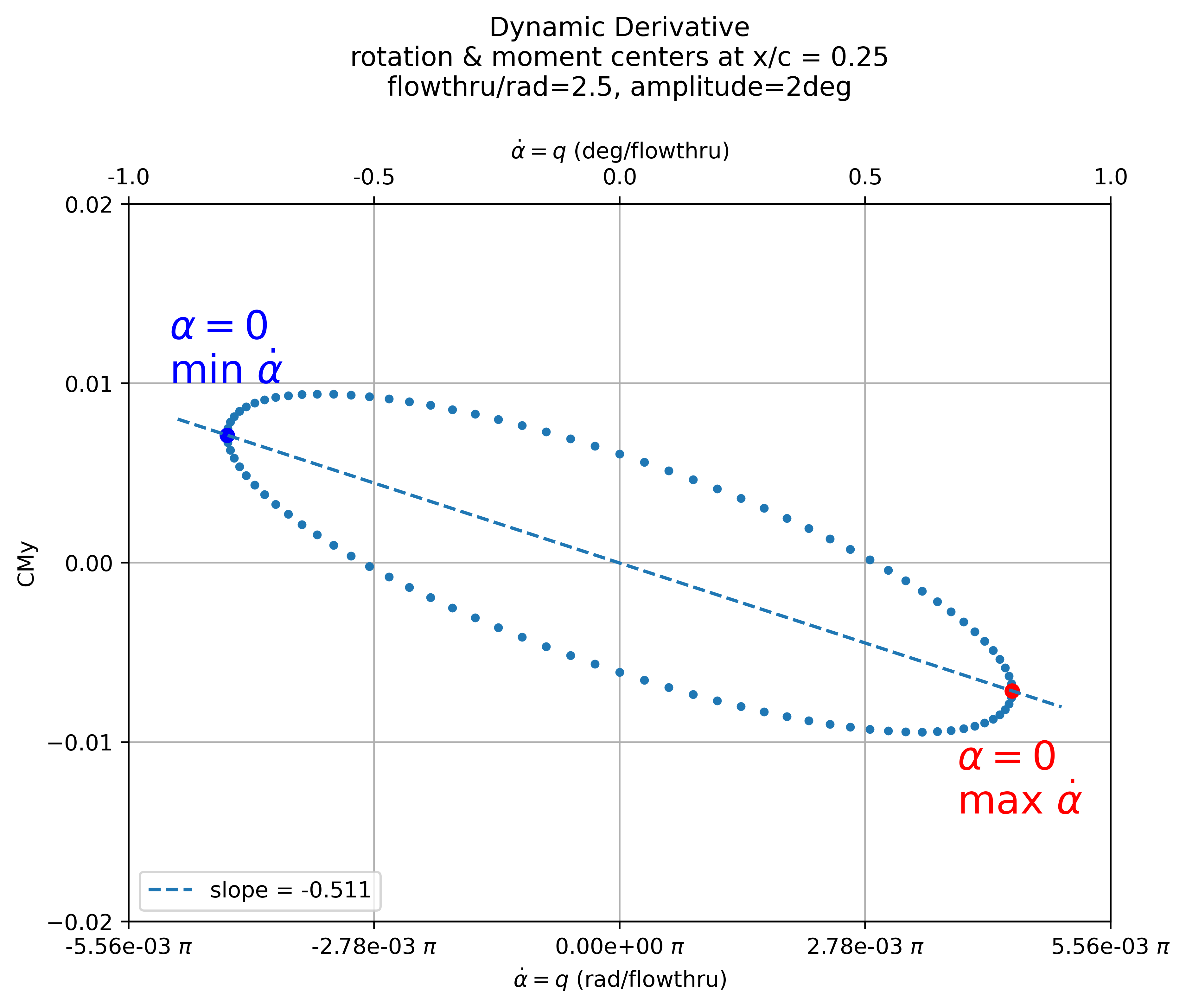
../../_images/CMy.png — Fig. 229 Dynamic Derivative $d C M y / d \dot{α}$ i.e. $d C M y / d q$ .#