Wall Model#
Introduction#
This case study presents and validates the wall model implemented within Flow360. Wall model simulations offer significant advantages over wall-resolved simulations leading to reductions in computational cost and speed improvements with limited impact on the simulation accuracy. Wall-resolved simulations typically require a
Wall Model Formulation in Flow360#
The wall model formulation in Flow360 is based on the concept of a wall velocity. Both the velocity at the wall and at the first grid point are updated during the solution process. From the solution, the ratio between the tangential velocities at the wall and first grid point is obtained (wallFunctionMetric can be output as part of the surface solution, with values below 1.25 indicating good estimation of the wall shear stress and values of above 10 meaning an unreliable estimation.
Flat Plate Case#
Simulation Setup#
The first case under consideration is the flat plate case, which is a canonical case often used for testing new implementations in CFD. The flat plate case is based on the model verification case available on the NASA TMR website. The freestream Mach number is equal to 0.2 with the Reynolds number per unit length equal to 5 million. The boundary conditions applied are based on the Flat Plate TMR Case, with the NoSlipWall boundary condition replaced with WallFunction for the wall model cases. The grids were generated based on the 137 by 97 nodes grid from the NASA TMR flat plate grids download page. This grid was loaded into a meshing tool and the wall spacing was modified to a number of values ranging from 4e-07 to 2e-03 to examine the effect of different
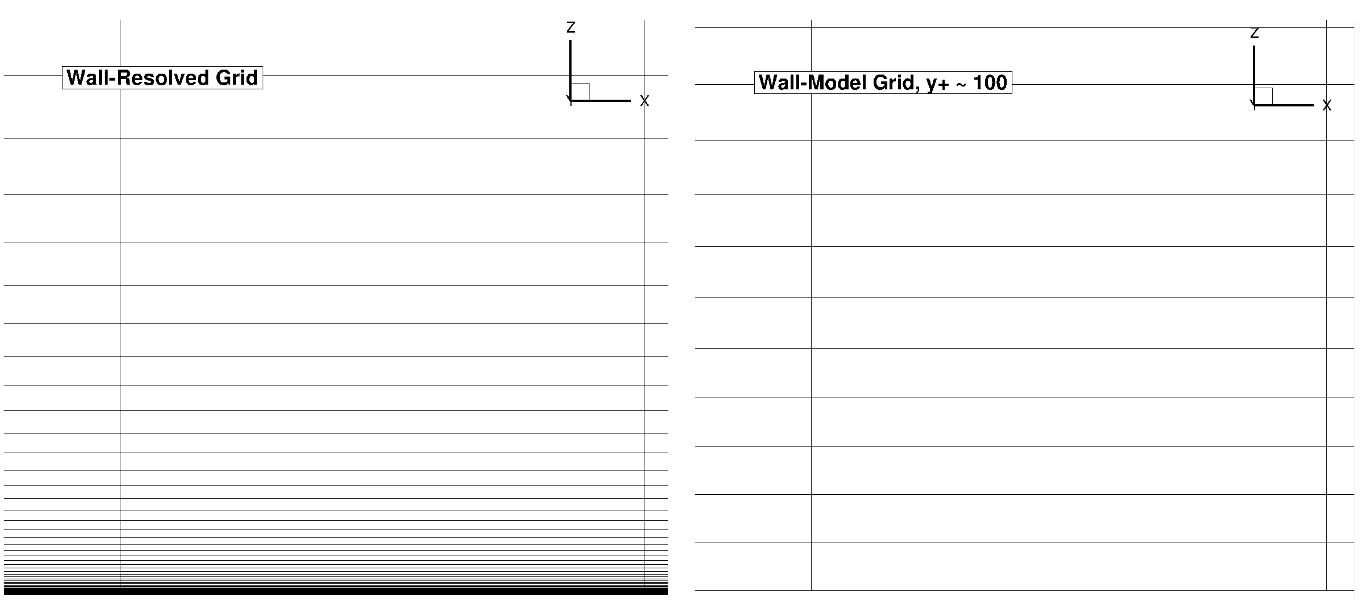
Fig. 81 Comparison of the wall-resolved (top) and wall-model (
As the number of points in the wall normal direction is fixed, the wall-model grid has a finer spacing away from the boundary layer due to the higher wall-normal spacing at the flat plate. The simulations were performed using both the Spalart-Allmaras and
Numerical Results#
Firstly, the drag values are compared across a range of wall spacings, shown in Table 13. The same data is shown in graphical format in Fig. 82.
Wall Spacing |
CD (Spalart-Allmaras) |
CD ( |
|
|---|---|---|---|
1E-06 (resolved) |
0.182 |
0.002846 |
0.002826 |
1E-06 |
0.176 |
0.002670 |
0.002654 |
4E-06 |
0.693 |
0.002581 |
0.002528 |
2E-05 |
3.25 |
0.002257 |
0.002139 |
4E-05 |
6.25 |
0.002077 |
0.001928 |
0.0001 |
16.3 |
0.002292 |
0.002090 |
0.0002 |
34.5 |
0.002544 |
0.002247 |
0.0004 |
68.3 |
0.002497 |
0.002398 |
0.0008 |
134 |
0.002423 |
0.002552 |
0.002 |
331 |
0.002373 |
0.002633 |
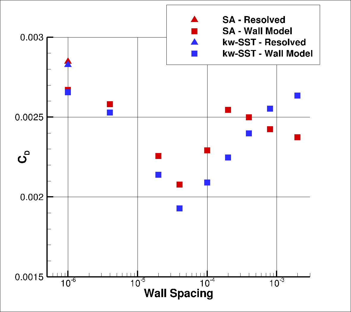
Fig. 82 Drag values for the flat plate case for a range of wall spacings for the Spalart-Allmaras and
As the wall spacing increases, the drag value is minorly underpredicted compared to the wall-resolved simulations, with the difference staying within 10% for the first two wall spacings. As the wall spacing is increased further, the error on the drag prediction increases, until spacings of 0.0002-0.0004 are reached, above which the error significantly reduces. Similar trends are observed between the Spalart-Allmaras and
.svg)

Fig. 83 Y+ values along the flat plate for wall-resolved (R) and wall-model simulations for the Spalart-Allmaras and
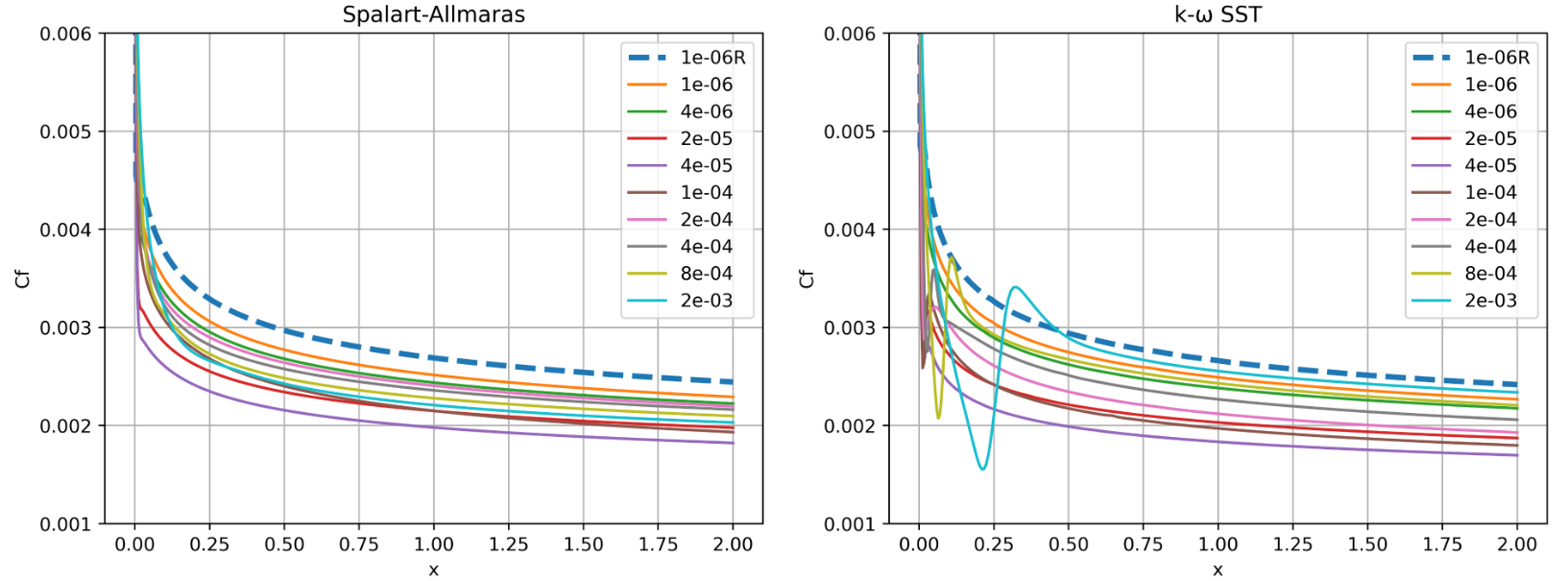
Fig. 84 Skin friction predictions along the flat plate for wall-resolved (R) and wall-model simulations for the Spalart-Allmaras and
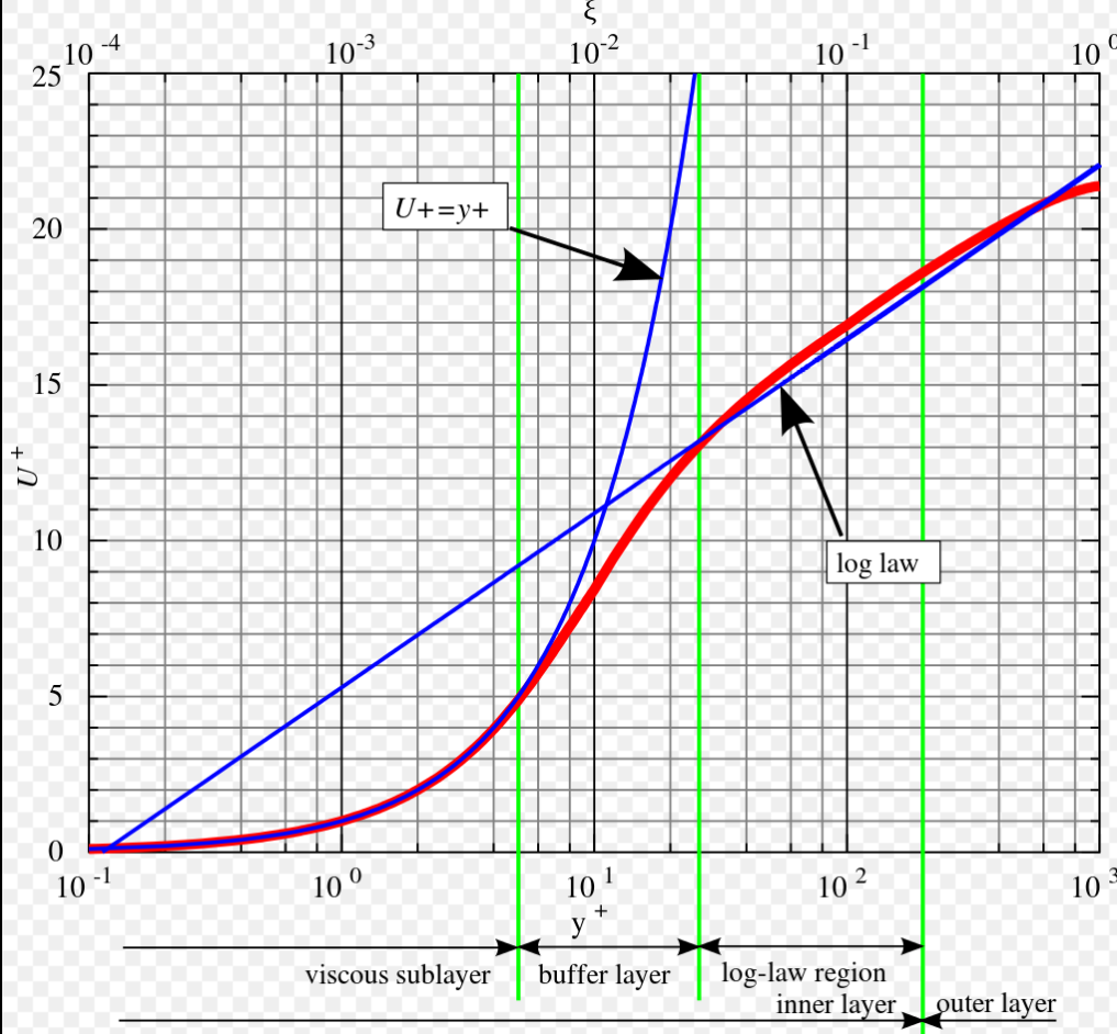
Fig. 85 Boundary layer profile in wall units according to the Law of the wall.#
The first observation is that the spacings with poorest agreement in drag have
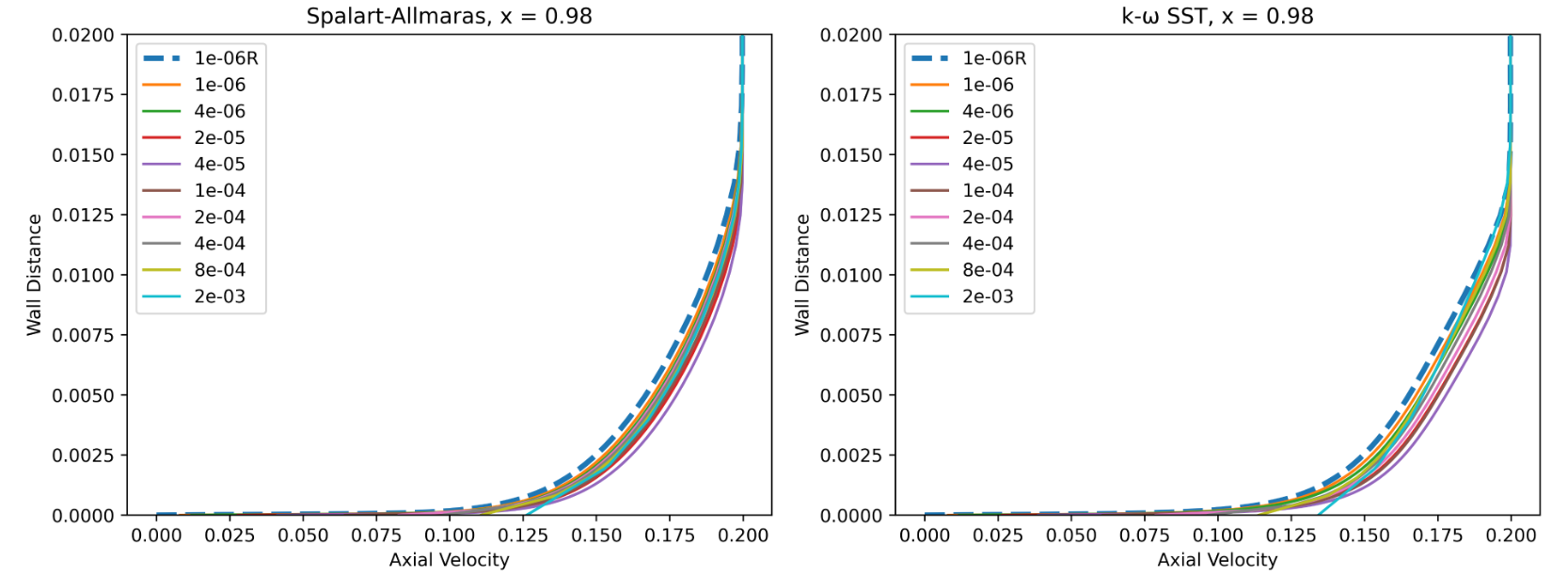
Fig. 86 Velocity profiles at x = 0.98 for wall-resolved (R) and wall-model simulations for the Spalart-Allmaras and
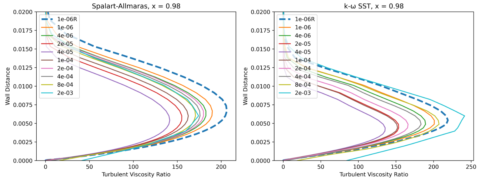
Fig. 87 Turbulence viscosity ratio at x = 0.98 for wall-resolved (R) and wall-model simulations for the Spalart-Allmaras and
The first observation is that for the wall model simulations, the axial velocity is non-zero at the wall as discussed in the wall model formulation. Very good agreement is obtained for the velocity profiles across a range of wall spacings, with the wall model simulations predicting a slightly higher velocity magnitude in the boundary layer. The poorest agreement is seen for wall spacings which are equivalent to the first layer thickness being in the buffer layer. Comparing the Spalart-Allmaras and
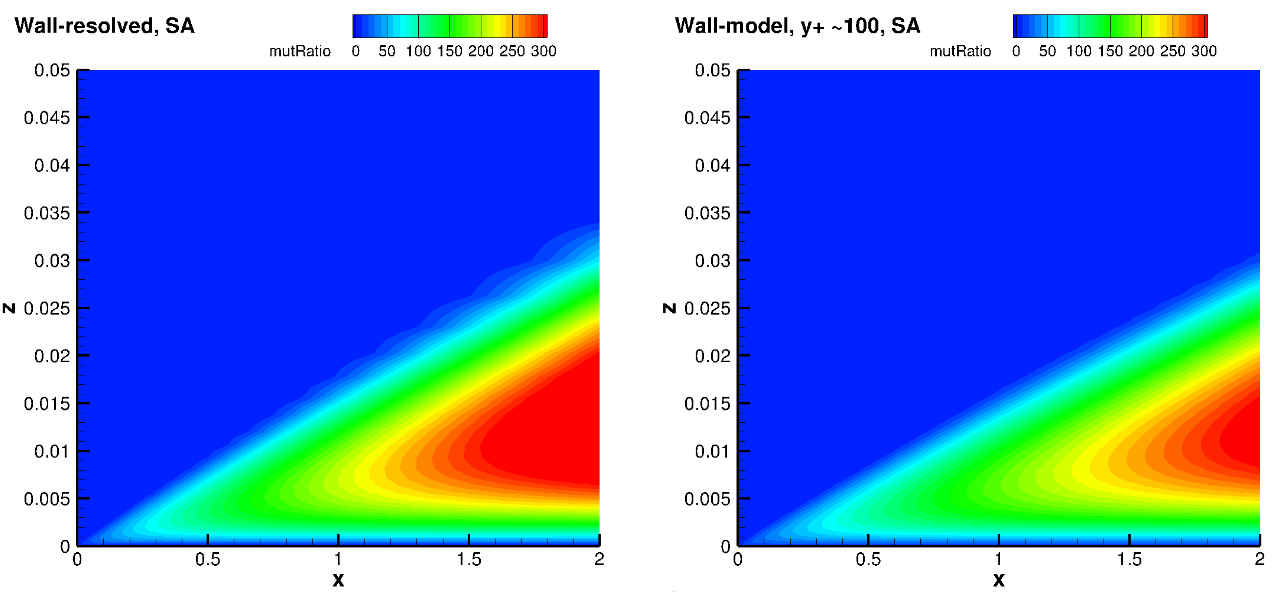

Fig. 88 Turbulence viscosity ratio fields for the wall-resolved (left) and wall-model at a
The turbulence eddy viscosity ratio fields show similar trends between wall-resolved and wall-model simulations. The peak eddy viscosity ratio is generally lower in the domain for the wall model simulations. The growth of eddy viscosity in the wall normal direction is lower for the
NACA0012 Case#
Simulation Setup#
The second case under consideration is the NACA0012 aerofoil at three angles of attack of
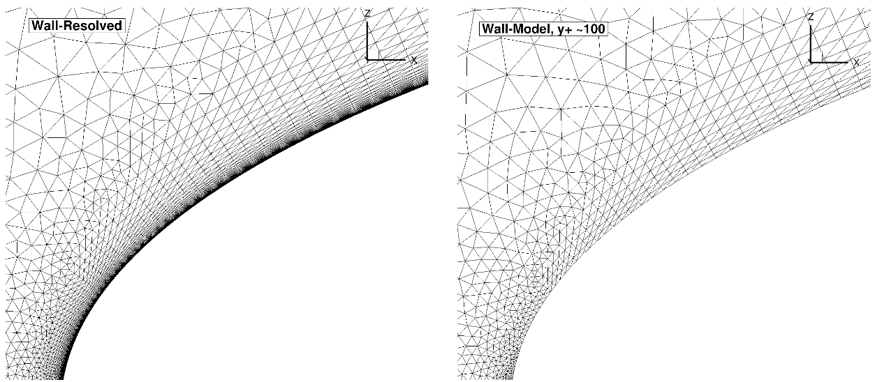
Fig. 89 Comparison of the wall-resolved (left) and wall-model (
The volumetric grids for the wall-resolved and wall-model grids look fairly similar when looking at the grid around the entire aerofoil. The wall-model grid for a
Numerical Results#
Firstly, the integrated loads are compared for wall-resolved and wall-model simulations. The integrated loads at an angle of attack of
Wall Spacing |
CL (Spalart-Allmaras) |
CL ( |
CD (Spalart-Allmaras) |
CD ( |
|---|---|---|---|---|
5E-07 (resolved) |
-0.0000358 |
-0.0000099 |
0.0081878 |
0.0082157 |
5E-07 |
-0.0000381 |
-0.0000148 |
0.0076578 |
0.0076832 |
2E-06 |
-0.0004925 |
-0.0005105 |
0.0074463 |
0.0073613 |
1E-05 |
-0.0002107 |
-0.0001959 |
0.0067913 |
0.0064732 |
2E-05 |
-0.0004692 |
-0.0004715 |
0.0062709 |
0.0058601 |
5E-05 |
-0.0003264 |
-0.0004367 |
0.0062592 |
0.0055318 |
0.0001 |
-0.0001271 |
-0.0001083 |
0.0072587 |
0.0060029 |
0.0002 |
-0.0000014 |
0.0000725 |
0.0074976 |
0.0062179 |
0.0004 |
0.0001888 |
0.0001342 |
0.0073109 |
0.0061955 |
0.001 |
-0.0003806 |
-0.0006551 |
0.0075675 |
0.0067801 |
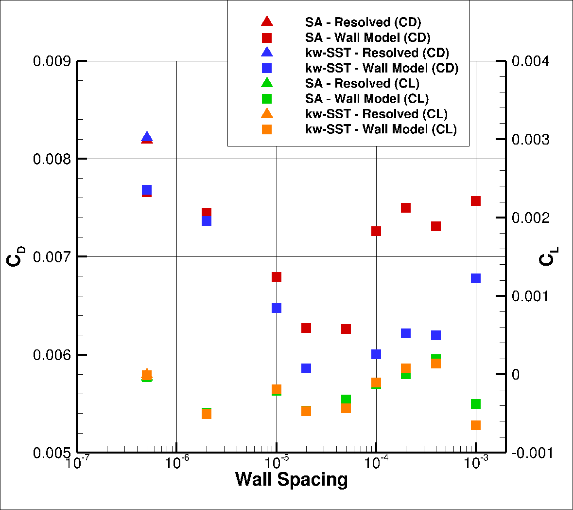
Fig. 90 Integrated loads values for the NACA0012 case at
At an angle of attack of
Wall Spacing |
CL (Spalart-Allmaras) |
CL ( |
CD (Spalart-Allmaras) |
CD ( |
|---|---|---|---|---|
5E-07 (resolved) |
1.0884010 |
1.0887404 |
0.0134051 |
0.0135129 |
5E-07 |
1.0954417 |
1.0961686 |
0.0125759 |
0.0126426 |
2E-06 |
1.0990507 |
1.1015714 |
0.0122834 |
0.0121173 |
1E-05 |
1.1111295 |
1.1166378 |
0.0110191 |
0.0104134 |
2E-05 |
1.1162736 |
1.1237324 |
0.0104958 |
0.0095929 |
5E-05 |
1.1099161 |
1.1213013 |
0.0112073 |
0.0098585 |
0.0001 |
1.0975726 |
1.1083656 |
0.0127432 |
0.0115825 |
0.0002 |
1.0891533 |
1.0946613 |
0.0137239 |
0.0133125 |
0.0004 |
1.0724442 |
1.0741733 |
0.0146291 |
0.0147813 |
0.001 |
1.0221160 |
1.0127430 |
0.0169448 |
0.0177315 |

Fig. 91 Integrated loads values for the NACA0012 case at
At a higher angle of attack of
Wall Spacing |
CL (Spalart-Allmaras) |
CL ( |
CD (Spalart-Allmaras) |
CD ( |
|---|---|---|---|---|
5E-07 (resolved) |
1.5297564 |
1.5185145 |
0.0251760 |
0.0260543 |
5E-07 |
1.5492167 |
1.5408299 |
0.0231829 |
0.0238758 |
2E-06 |
1.5628159 |
1.5627701 |
0.0221807 |
0.0221119 |
1E-05 |
1.5935174 |
1.6096414 |
0.0192190 |
0.0176531 |
2E-05 |
1.5974993 |
1.6213546 |
0.0188605 |
0.0164618 |
5E-05 |
1.5631734 |
1.5867074 |
0.0222658 |
0.0198286 |
0.0001 |
1.5170764 |
1.4840374 |
0.0274184 |
0.0306383 |
0.0002 |
0.7113100 |
0.7217588 |
0.1765999 |
0.1793623 |
0.0004 |
0.7508150 |
0.7638725 |
0.1655428 |
0.1669165 |
0.001 |
0.9306330 |
0.8796866 |
0.1159778 |
0.1310237 |
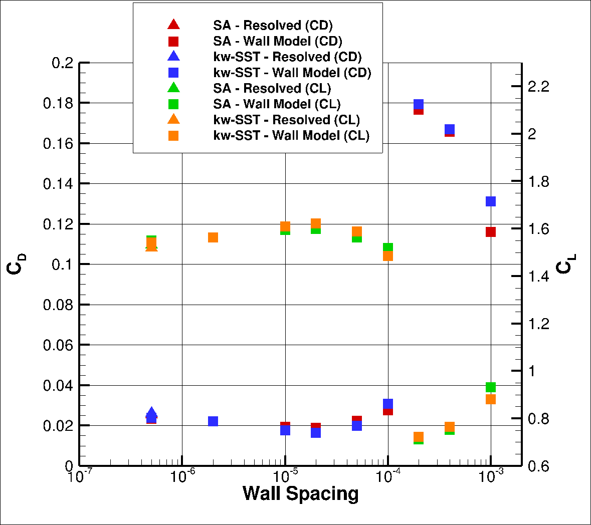
Fig. 92 Integrated loads values for the NACA0012 case at
At the highest angle of attack of
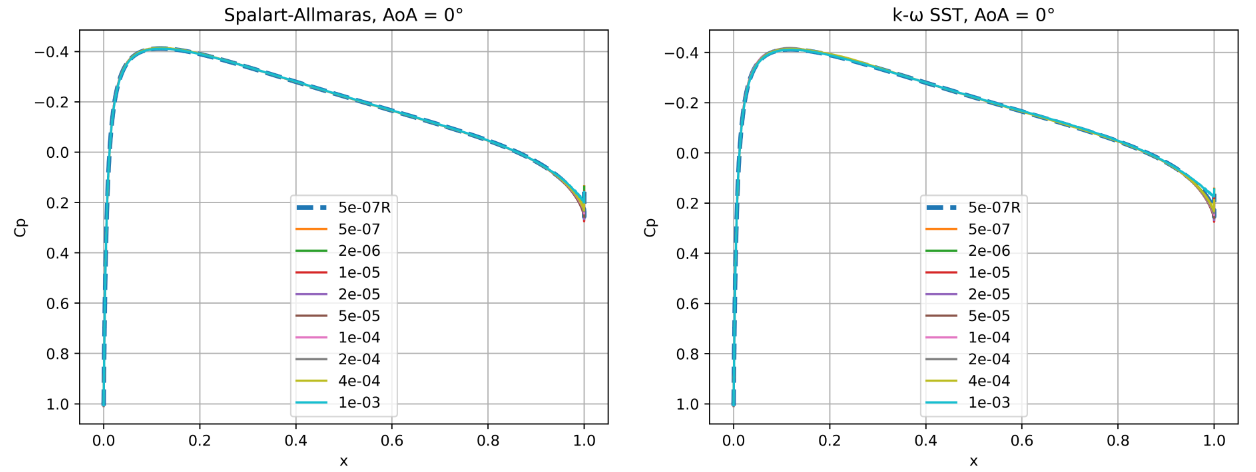

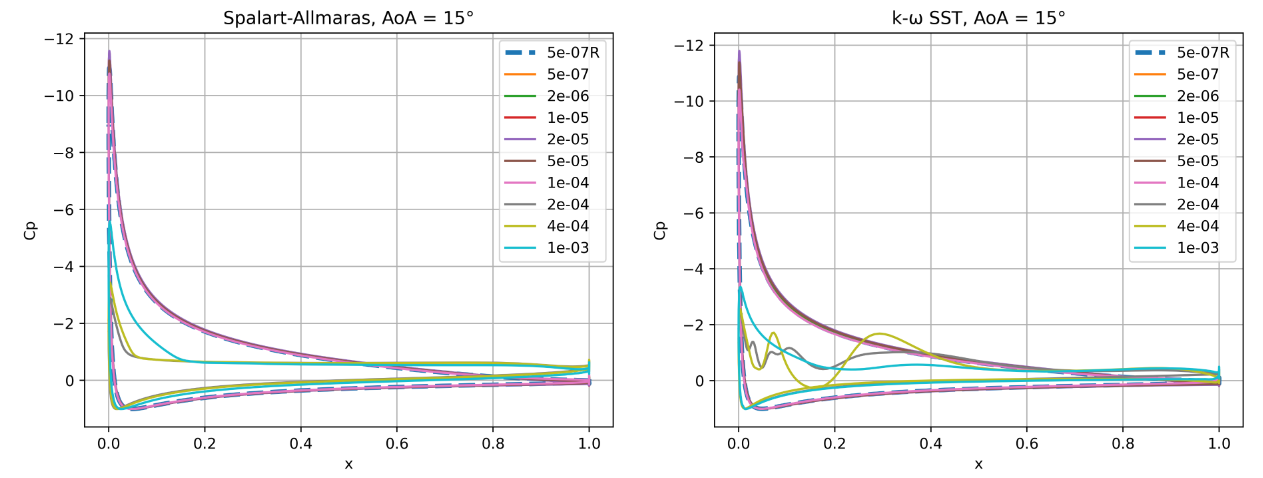
Fig. 93 Surface pressure coefficient predictions for the NACA0012 case for wall-resolved (R) and wall-model simulations at three angles of attack for the Spalart-Allmaras and
At an angle of attack of


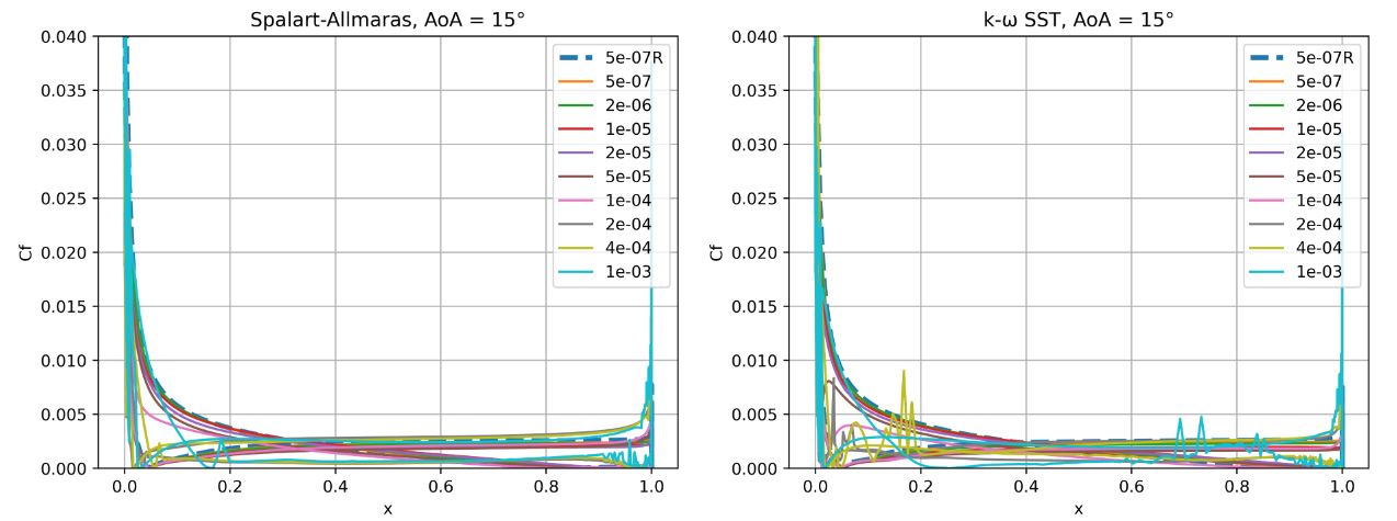
Fig. 94 Skin friction coefficient predictions for the NACA0012 case for wall-resolved (R) and wall-model simulations at three angles of attack for the Spalart-Allmaras and
The skin friction coefficient curves indicate greater differences between the two turbulence models. At an angle of attack of
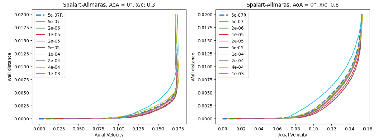
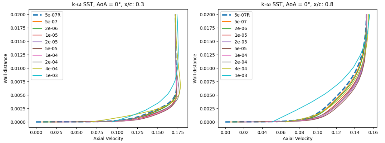

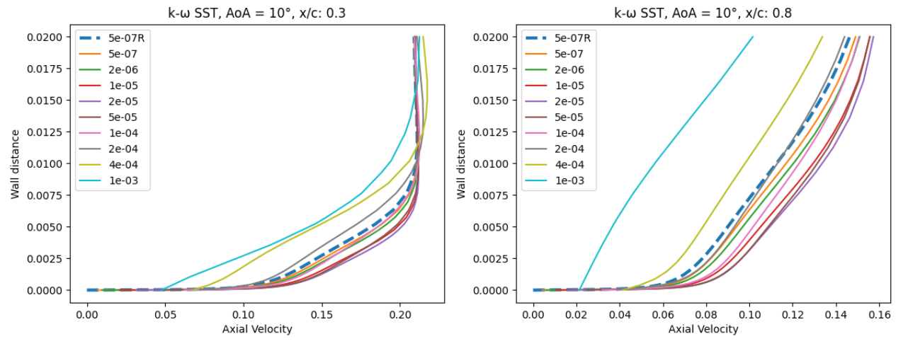
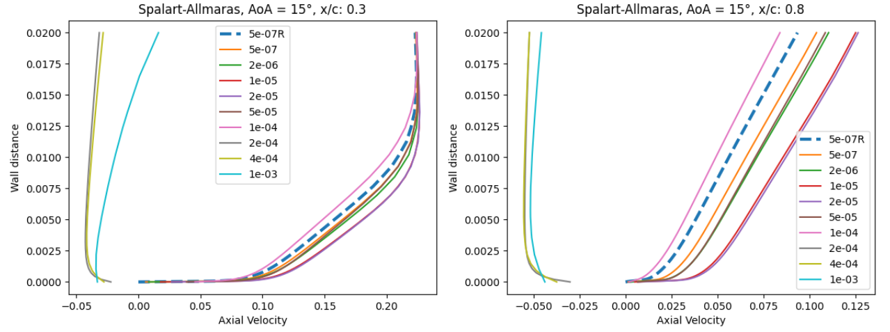
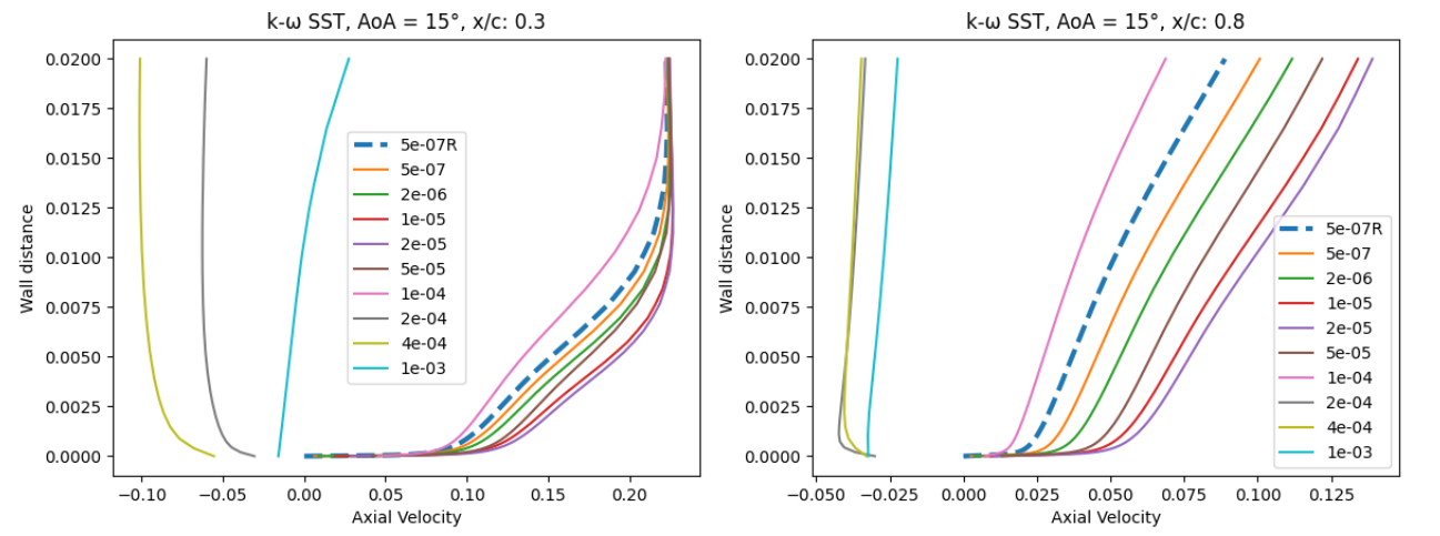
Fig. 95 Velocity profile predictions for the NACA0012 case for wall-resolved (R) and wall-model simulations at three angles of attack and two chordwise locations for the Spalart-Allmaras and
At an angle of attack of
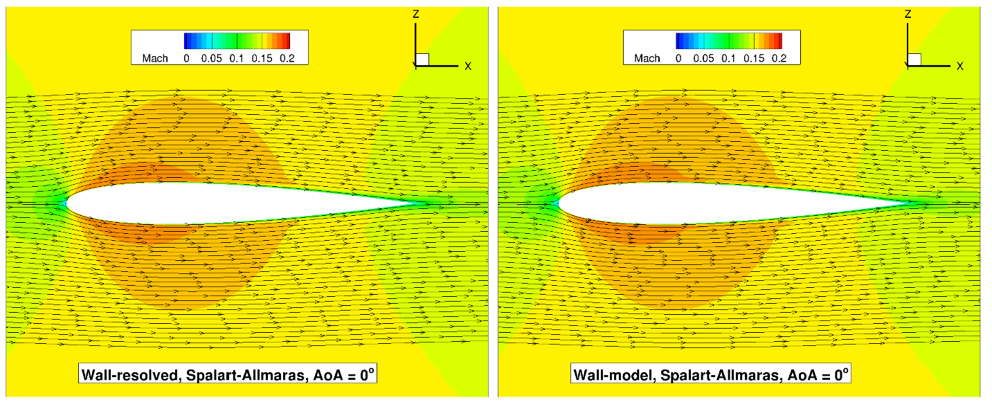

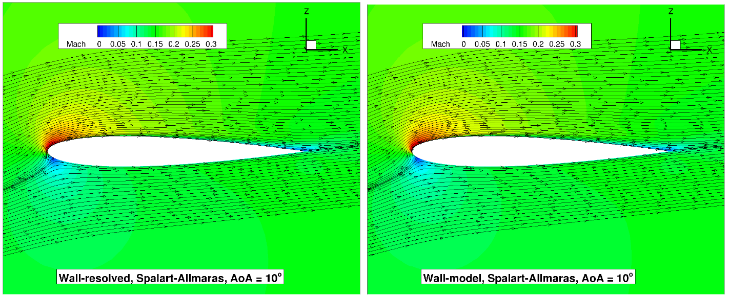

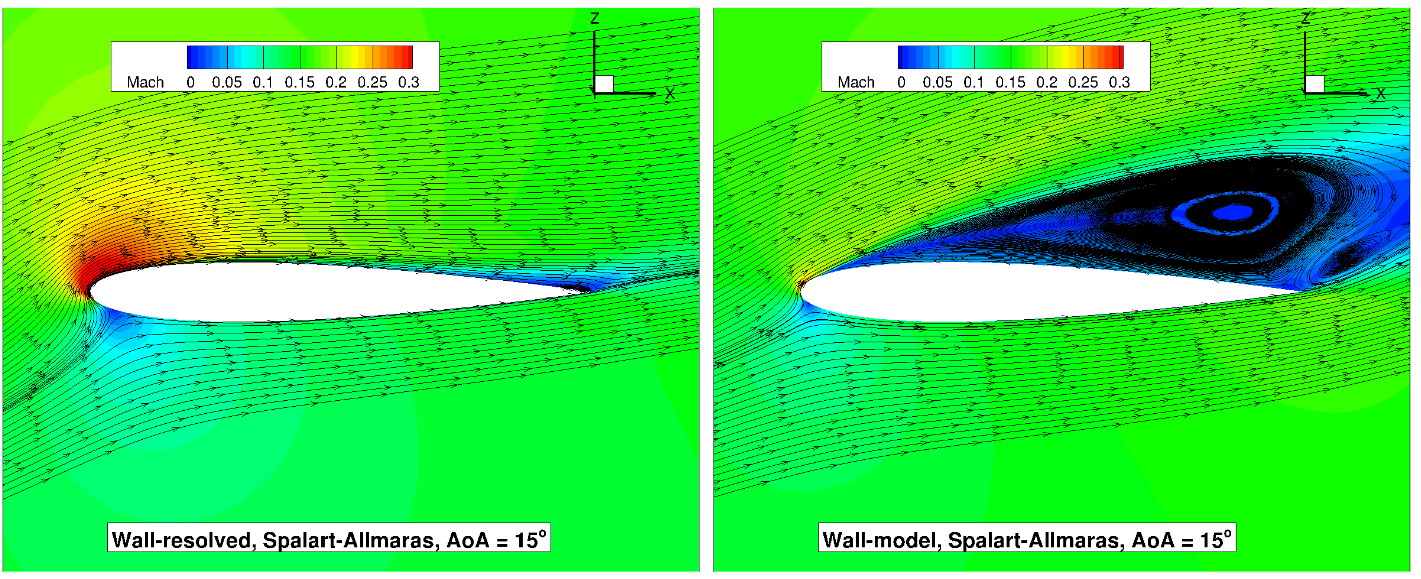

Fig. 96 Volume streamlines for the NACA0012 case for wall-resolved (R) and wall-model (at ~100
The flowfield streamlines show a very similar flowfield at
ONERAM6 Wing Case#
Simulation Setup#
The next case under consideration is the ONERAM6 wing case in transonic conditions. This case aims to evaluate the wall model for a 3D configuration in the presence of a shock-induced separation and strong pressure gradients. The ONERAM6 wing case is a standard CFD validation case for transonic flows, with the results from wall-resolved simulations using Flow360 available in the ONERAM6 wing case study. The flow conditions under consideration are a Mach number of 0.84, Reynolds number based on MAC of 11.72 million at an angle of attack of 3.06 degrees. The grids were generated using our automated meshing workflow. The surface grid for this case is shown in Fig. 97.
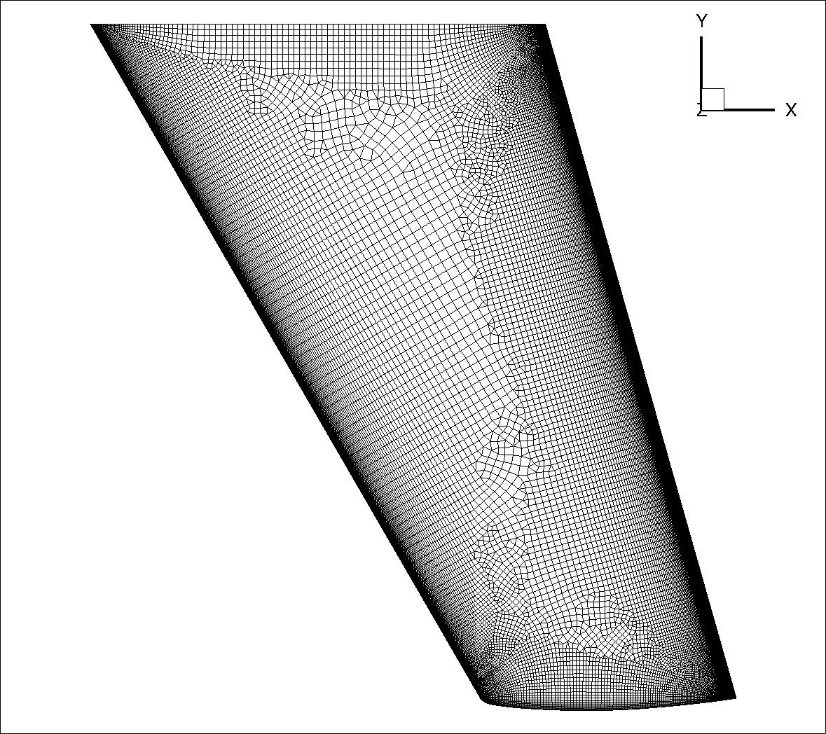
Fig. 97 ONERAM6 wing surface grid used for the wall-resolved and wall-model simulations.#
The surface grid is fixed for both wall-resolved and wall-model simulations. The surface grid has 86,280 nodes. Anisotropic layers are grown from the the leading and trailing edges, to resolve the areas of the flow with strong flow gradients, although no attempt is made to refine the mesh near the shock. A set of volume grids were generated with spacing values ranging from 5e-07 to 1e-03, leading to grids ranging from 15.3 million nodes to 2.3 million nodes. A slice through the volume at the wing mid-span of the wall-resolved grid and wall model grid with a wall spacing of 2e-04 (approximately

Fig. 98 Comparison of the wall-resolved (top) and wall-model (
Similarly to the NACA0012 airfoil, from this view, the wall-model and wall-resolved grids look very similar, although the wall model grid has fewer anisotropic layers leading to a reduction in node counts from 15.3 million to 4.8 million. The simulations were performed using both the Spalart-Allmaras and
Numerical Results#
Firstly, the integrated loads are compared for wall-resolved and wall-model simulations for both examined turbulence models, shown in Table 17. The same data is shown in graphical format in Fig. 99
Wall Spacing |
CL (Spalart-Allmaras) |
CL ( |
CD (Spalart-Allmaras) |
CD ( |
|---|---|---|---|---|
5E-07 (resolved) |
0.2745839 |
0.2709627 |
0.0174882 |
0.0173155 |
5E-07 |
0.2750711 |
0.2716485 |
0.0172173 |
0.0170549 |
2E-06 |
0.2753277 |
0.2724487 |
0.0170231 |
0.0167591 |
1E-05 |
0.2765591 |
0.2750969 |
0.0162665 |
0.0158812 |
2E-05 |
0.2771044 |
0.2761809 |
0.0160069 |
0.0155393 |
5E-05 |
0.2744205 |
0.2733292 |
0.0170425 |
0.0162485 |
0.0001 |
0.2727455 |
0.2711933 |
0.0173144 |
0.0166847 |
0.0002 |
0.2726556 |
0.2689671 |
0.0172488 |
0.0171784 |
0.0004 |
0.2718576 |
0.2657272 |
0.0171138 |
0.0175339 |
0.001 |
0.2701289 |
0.0171885 |
||
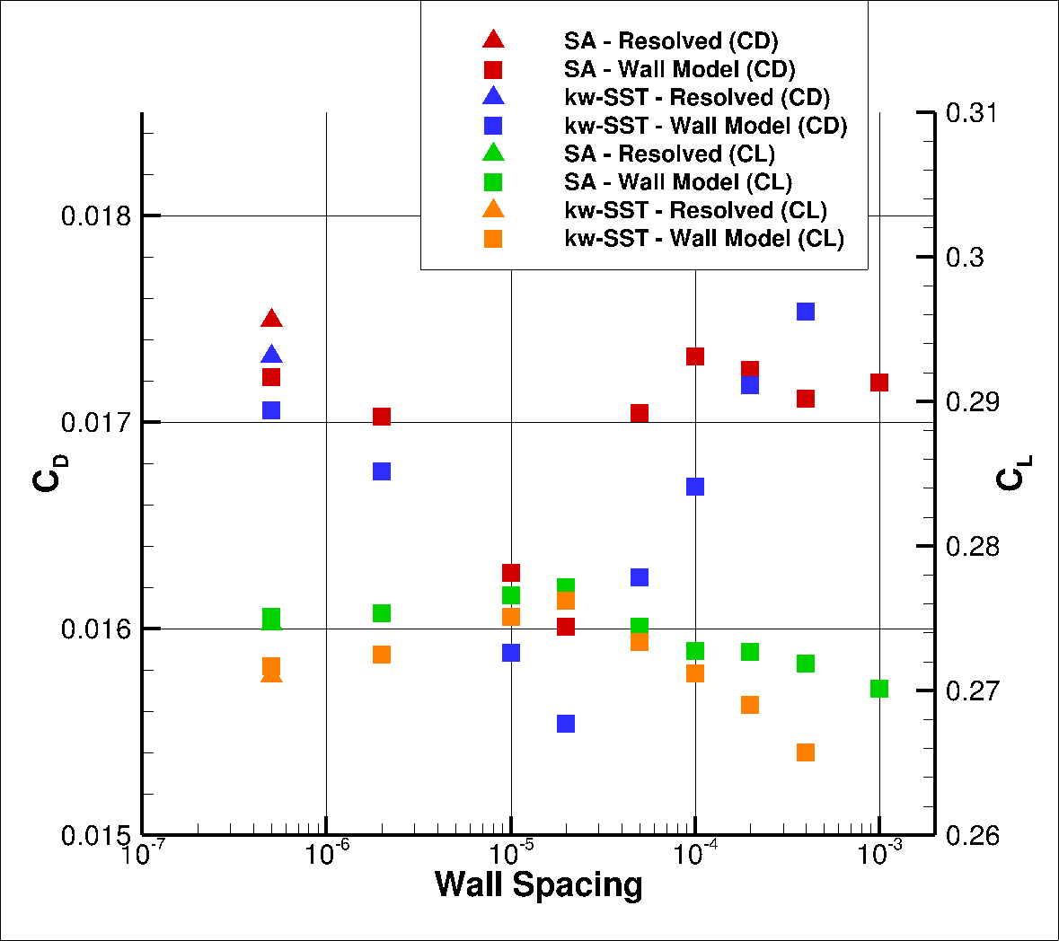
Fig. 99 Integrated loads values for the ONERAM6 case for a range of wall spacings for the Spalart-Allmaras and
The wall model simulations for this case show excellent agreement with wall-resolved simulations, across the examined wall spacings. Similarly as for the NACA0012 airfoil cases, at low wall spacings the agreement is quite close and reduces as the spacing is increased in both lift and drag, with the lift being slightly overpredicted and drag being slightly underpredicted. The agreement significantly improves at wall spacings of 5e-05 to 0.0004. For a wall spacing of 2e-04, the lift and drag predictions are within 1% of the wall resolved simulations for both turbulence models. To examine this in greater detail, the

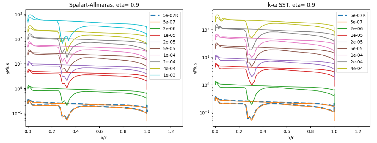
Fig. 100 Y+ values along the ONERAM6 wing for wall-resolved (R) and wall-model simulations at two spanwise locations for the Spalart-Allmaras and
The


Fig. 101 Surface pressure coefficient predictions for the ONERAM6 wing case for wall-resolved (R) and wall-model simulations at two spanwise locations for the Spalart-Allmaras and
The surface pressure predictions at the two spanwise locations, show a very low sensitivity to wall spacing. At eta=0.44 two shocks are present along the chordwise direction, whereas at eta=0.9 a single strong shock is located at approximately x/c=0.3. The use of the wall model appears to have a minor impact on the shock locations, but also leads to a poorer resolution of the shock at high wall spacing. The skin friction predictions are shown in Fig. 102.
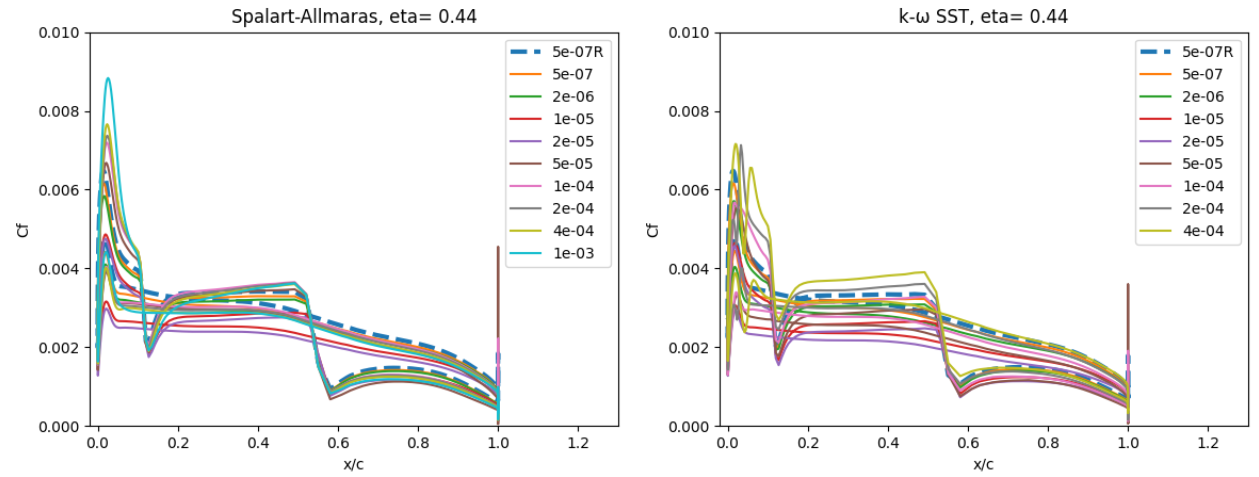
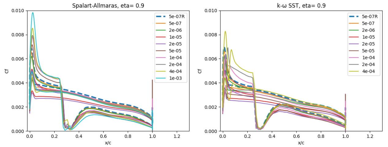
Fig. 102 Skin friction coefficient predictions for the ONERAM6 wing case for wall-resolved (R) and wall-model simulations at two spanwise locations for the Spalart-Allmaras and
A slightly higher sensitivity is seen for the surface skin friction. At eta=0.44, the skin friction is underpredicted at low wall spacings and overpredicted at high wall spacings, which is especially visible ahead of the first shock as the flow accelerates over the leading edge of the wing section. The general skin friction distribution trend, however, is captured well across all wall spacings. Similar observations can be made at the section near the wing tip. The Spalart-Allmaras and
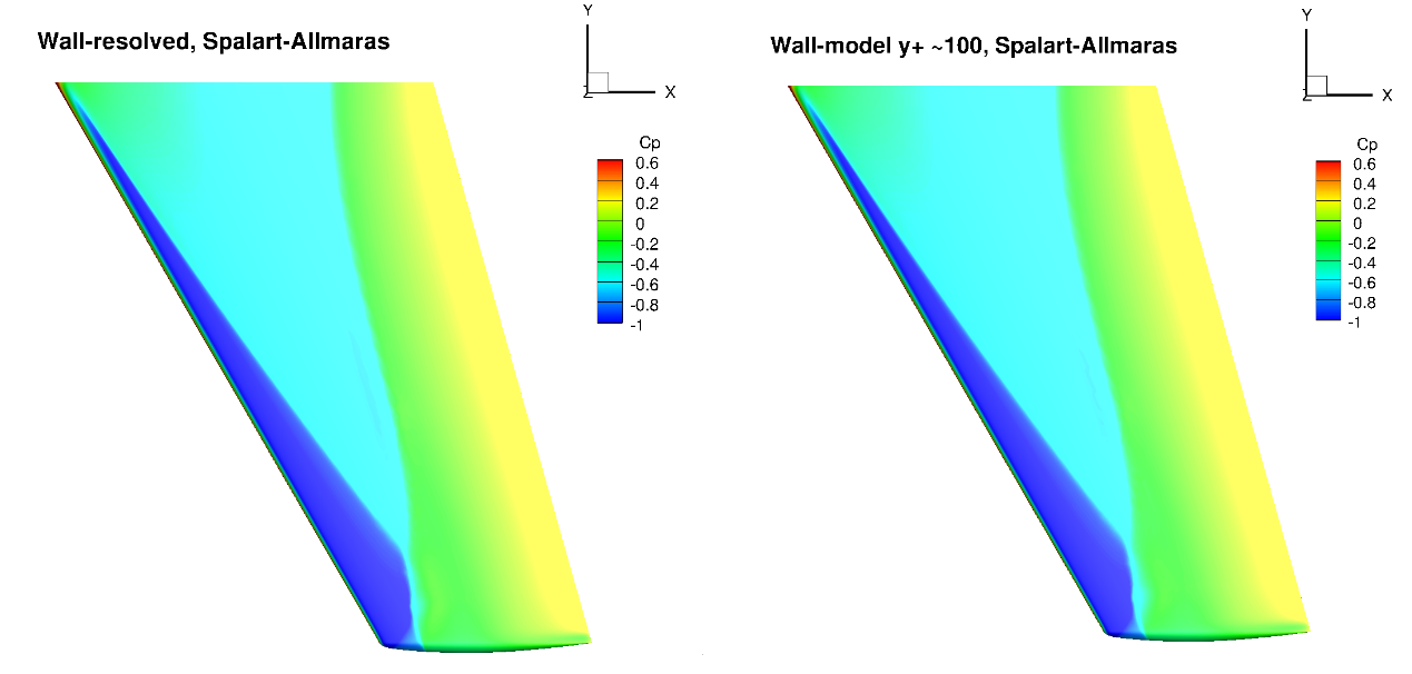
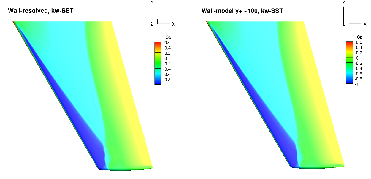
Fig. 103 Surface pressure coefficient predictions for the ONERAM6 wing case for wall-resolved (R) and wall-model (~100
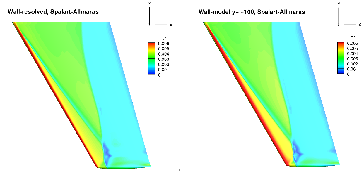
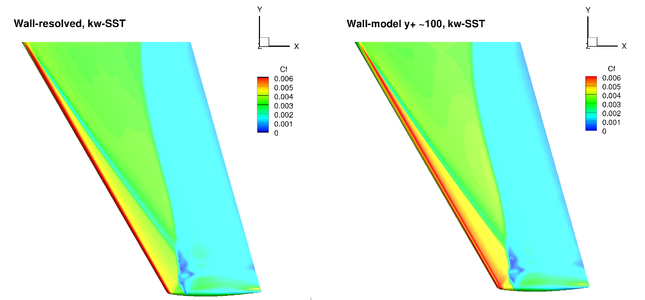
Fig. 104 Surface skin friction coefficient predictions for the ONERAM6 wing case for wall-resolved (R) and wall-model (~100
The surface pressure distributions across the entire wing show a very high degree of consistency for the wall-resolved and wall-model simulations and both turbulence models. This shows the high quality of the solution coming from the wall model. The skin friction distributions are also very similar with the wall-model simulations predicting a slightly higher skin friction magnitude near the leading edge and over a larger portion of the chord, across the entire wing. There are also minor differences in the shock-induced separation region. To examine these findings further we extracted the velocity profiles at the two spanwise locations (eta=0.44 and 0.9) and two chordwise locations of x/c=0.3 ad 0.8, shown in Fig. 105.
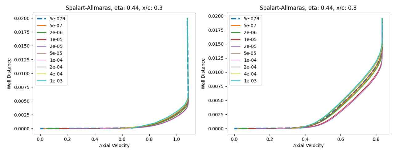
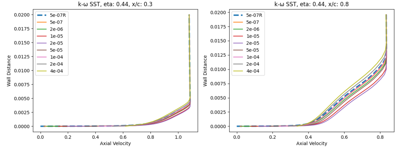
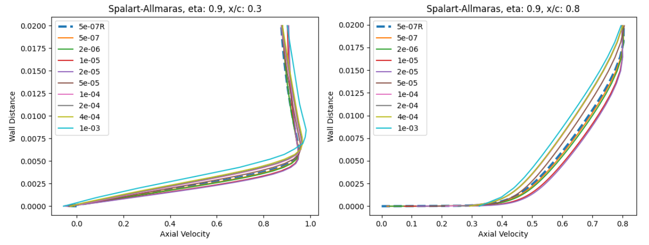

Fig. 105 Velocity profile predictions for the ONERAM6 wing case for wall-resolved (R) and wall-model simulations at two spanwise and two chordwise locations for the Spalart-Allmaras and
At eta=0.44 and x/c=0.3, the velocity profiles show good agreement across all wall spacings when compared to the wall-resolved simulations, with the largest errors present at wall-spacings of 1e-05 to 2e-05 which are in the buffer region. Further downstream at x/c=0.8 slightly greater differences are observed, especially for the wall spacings in the buffer region, with higher predicted axial velocity magnitudes. The trends are similar for both turbulence models. Further outboard at eta=0.9, similar observations can be made, although the highest wall spacings now also lead to some differences. Here, the highest wall spacing leads to an underprediction of the axial velocity across the boundary layer. A small pocket of separated flow can also be noticed at x/c=0.3 which is well captured by the wall model.
Ahmed Body Case#
Simulation Setup#
The next case under consideration is the Ahmed body case, which is often used as the baseline case for validation in automotive applications, making it a great starting point for wall model validation for automotive cases. The flow conditions under consideration are a Mach number of 0.1728 with a Reynolds number of 4.176 million. The inlet and outlet boundaries are set to farfield with the floor also modeled as a no slip wall or using the wall function approach. The grids were generated by starting from a structured surface grid, and manually generating the volume grids. The surface grid for this case is shown in Fig. 106.
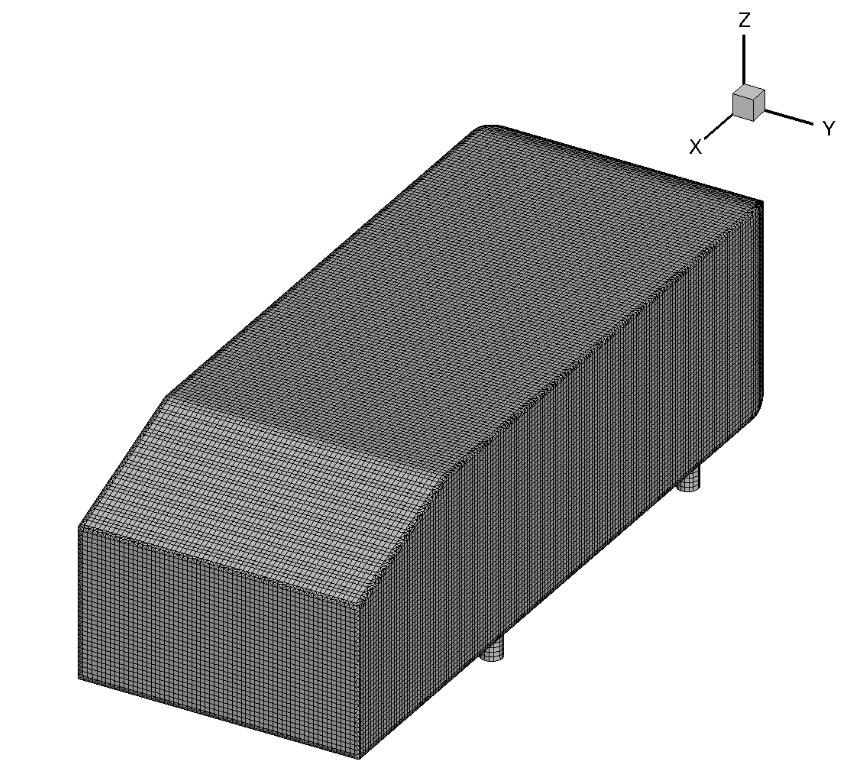
Fig. 106 Ahmed body surface grid used for the wall-resolved and wall-model simulations.#
The surface grid is fixed for both wall-resolved and wall-model simulations. The surface grid has 39,434 nodes. The spacing is fairly uniform over the entire vehicle. A set of volume grids were generated with spacing values ranging from 5e-07 to 1e-03, leading to grids ranging from 3 million nodes to 0.85 million nodes. A slice through the volume along the centerline of the wall-resolved grid and wall model grid with a wall spacing of 4e-04 (approximately

Fig. 107 Comparison of the wall-resolved (top) and wall-model (
From this view, the wall-model and wall-resolved grids look very similar, similarly as in the previously examined cases. The wall model grid has fewer anisotropic layers leading to a reduction in node counts from 3 million to 1.1 million. The simulations were performed using both the Spalart-Allmaras and
Numerical Results#
Firstly, the integrated loads are compared for wall-resolved and wall-model simulations for both examined turbulence models, shown in Table 18. The same data is shown in graphical format in Fig. 108
Wall Spacing |
CL (Spalart-Allmaras) |
CL ( |
CD (Spalart-Allmaras) |
CD ( |
|---|---|---|---|---|
5E-07 (resolved) |
0.2838657 |
0.2727445 |
0.3389527 |
0.3246567 |
5E-07 |
0.2833976 |
0.2723599 |
0.3351060 |
0.3203302 |
2E-06 |
0.2815923 |
0.2708006 |
0.3346436 |
0.3197694 |
1E-05 |
0.2817096 |
0.2777542 |
0.3308835 |
0.3120820 |
2E-05 |
0.2789197 |
0.2757056 |
0.3277845 |
0.3087600 |
5E-05 |
0.2772840 |
0.2669671 |
0.3248126 |
0.3031932 |
0.0001 |
0.2811986 |
0.2701703 |
0.3305484 |
0.3151284 |
0.0002 |
0.2895193 |
0.2832801 |
0.3410175 |
0.3253558 |
0.0004 |
0.2936916 |
0.2885895 |
0.3483039 |
0.3300952 |
0.001 |
0.2936290 |
0.3219432 |
0.3620031 |
0.3477800 |

Fig. 108 Integrated loads values for the Ahmed case for a range of wall spacings for the Spalart-Allmaras and
The integrated loads show excellent agreement for the wall-model simulations when compared to the wall-resolved simulations. At low wall spacings, both the lift and drag coefficients decreases with increasing wall spacing, until a spacing of 5e-05. At a spacing of 0.0001 both the drag and lift start to increase with excellent agreement with the wall-resolved simulations, which slightly worsens at the highest examined wall spacing. The best agreement is seen at a wall spacing of 0.0001 for the Spalart-Allmaras turbulence model and 0.0002 for the
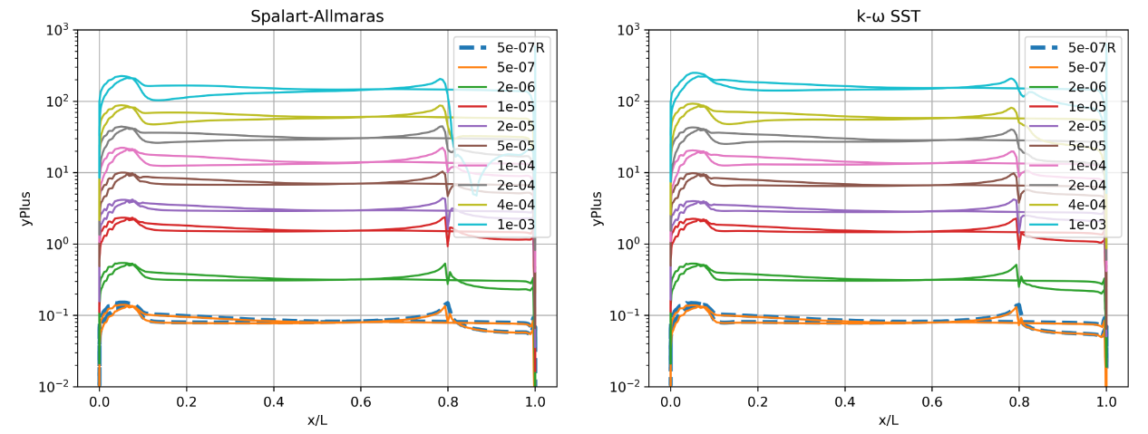
Fig. 109 Y+ values along the centerline (y=0) of the Ahmed body for wall-resolved (R) and wall-model simulations for the Spalart-Allmaras and
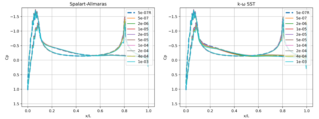
Fig. 110 Surface pressure predictions along the centerline (y=0) of the Ahmed body for wall-resolved (R) and wall-model simulations for the Spalart-Allmaras and
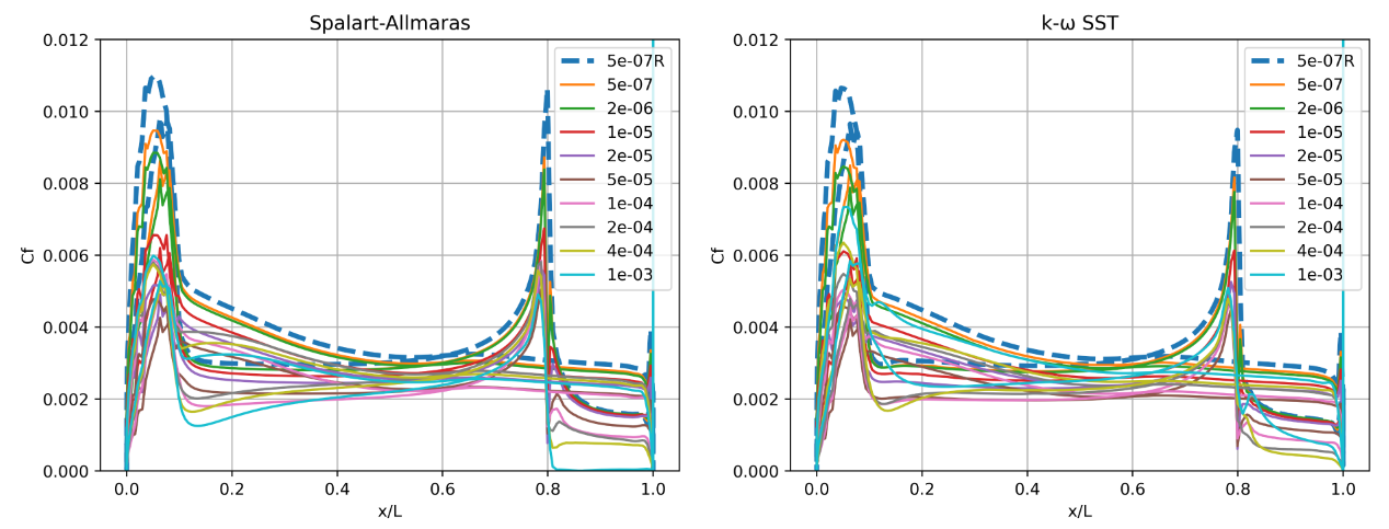
Fig. 111 Skin friction predictions along the centerline (y=0) of the Ahmed body for wall-resolved (R) and wall-model simulations for the Spalart-Allmaras and
Based on the
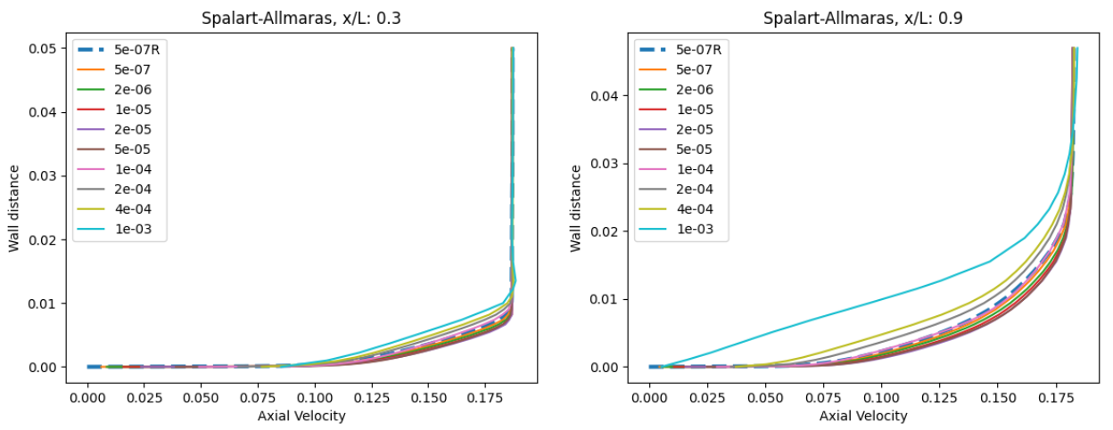
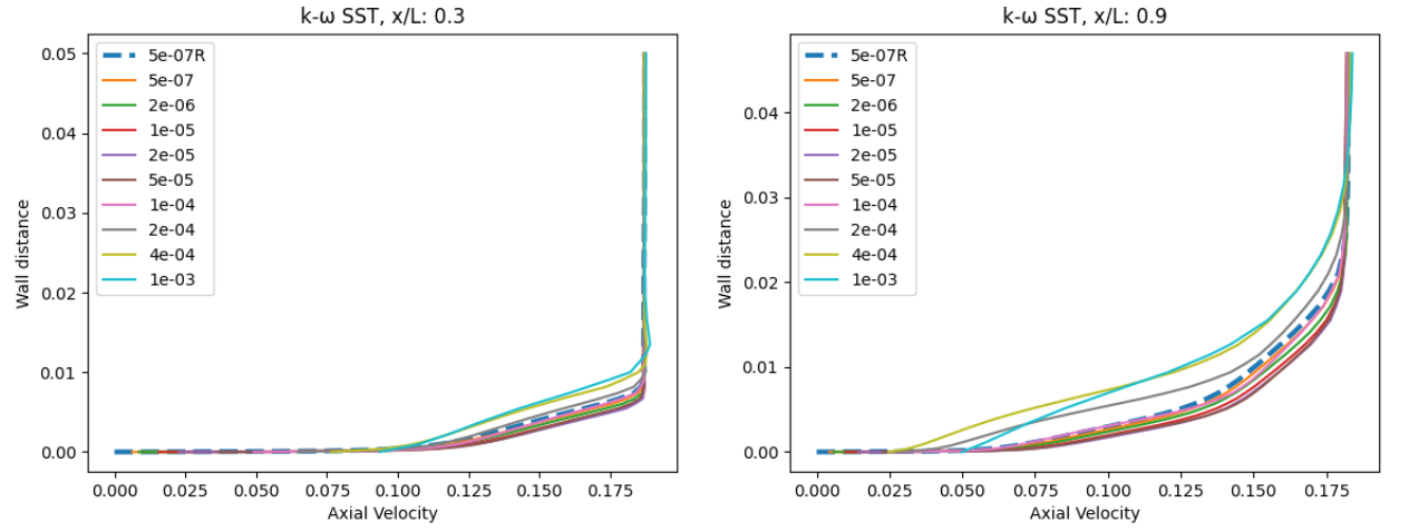
Fig. 112 Velocity profile predictions for the Ahmed body case for wall-resolved (R) and wall-model simulations at two locations along the centerline (y=0) for the Spalart-Allmaras and
At x/L=0.3, the velocity profiles are consistent for most wall spacings, with the axial velocity slightly decreasing with increasing wall spacing. The differences are slightly higher for the


Fig. 113 Flowfield predictions along the centerline (y=0) for the Ahmed body case for wall-resolved (R) and wall-model (at ~100
Qualitatively, the flowfield streamlines show excellent agreement between wall-resolved and wall-modeled simulations for both examined turbulence models. Although the flow at the back of the car, was not the focus of this study, similar flow features are observed with a larger and smaller recirculation region present. The highly consistent flowfields highlight the applicability of the wall model to automotive applications.
Windsor Body Case#
Simulation Setup#
The final case under consideration is the Windsor body case, which is also aimed at automotive applications. This case was used during the 2nd automotive prediction workshop, and hence is seen as a more realistic automotive test case. The flow conditions under consideration are a Mach number of 0.1175 and Reynolds number of 0.77 million based on the vehicle height. The boundary conditions setup is similar to the Ahmed body case, with the floor modeled as a no slip wall or using wall functions. Only half the vehicle is modeled with a symmetry plane used at the vehicle centerline. The grids were generated using ANSA, with the surface grid shown in Fig. 114.
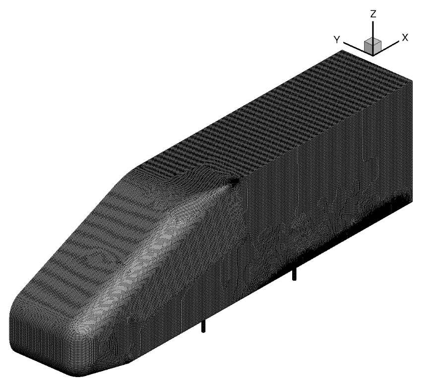
Fig. 114 Windsor body surface grid used for the wall-resolved and wall-model simulations.#
The surface grid used for both wall-resolved and wall-model simulations is fairly fine and has 152,601 nodes for a half-body. The spacing is fairly uniform over the entire vehicle. A set of volume grids were generated with spacing values ranging from 1e-06 to 2.5e-03, leading to grids ranging from 7.3 million nodes to 2.7 million nodes. The volumetric grid along the symmetry plane for the wall-resolved and wall model grids (spacing of 4e-04, approximately

Fig. 115 Comparison of the wall-resolved (top) and wall-model (
For the Windsor body cases, the number of anisotropic layers was adjusted manually. 25 layers were used for the wall-resolved simulations, which were gradually reduced to 9 layers for the mesh with the highest wall spacing. Here, the differences in the mesh near the wall can be seen clearly, with a prism layers extending deeper into the domain for the wall model grid. For the same height of the anisotropic region, even more layers would need to be used for the wall-resolved mesh. Compared to the automotive prediction workshop grids, no attempt was made at refining the mesh at the rear of the car, as the focus here is on evaluating the wall model rather than direct comparisons with experimental data. The wall model grid shown above, leads to a reduction in node counts from 7.3 million to 3.1 million nodes. The simulations were performed using both the Spalart-Allmaras and
Numerical Results#
Firstly, the integrated loads are compared for wall-resolved and wall-model simulations for both examined turbulence models, shown in Table 19.
Wall Spacing |
CL (Spalart-Allmaras) |
CL ( |
CD (Spalart-Allmaras) |
CD ( |
|---|---|---|---|---|
1e-06 (resolved) |
-0.1491836 |
-0.1095171 |
0.3453143 |
0.2940736 |
1e-06 |
-0.1531223 |
-0.1118958 |
0.3424746 |
0.2886777 |
5e-06 |
-0.1558363 |
-0.1216370 |
0.3413276 |
0.2886765 |
2.5e-05 |
-0.1631274 |
-0.1230071 |
0.3389714 |
0.2818219 |
5e-05 |
-0.1688174 |
-0.1260008 |
0.3392483 |
0.2820035 |
1.25e-04 |
-0.1721921 |
-0.1308088 |
0.3427992 |
0.2815498 |
2.5e-04 |
-0.1580500 |
-0.1195373 |
0.3543502 |
0.2915398 |
5e-04 |
-0.1606261 |
-0.1169904 |
0.3637310 |
0.3032360 |
1e-04 |
-0.1716058 |
-0.1234653 |
0.3781859 |
0.3180197 |
2.5e-03 |
-0.1687491 |
-0.1135775 |
0.4028245 |
0.3452181 |
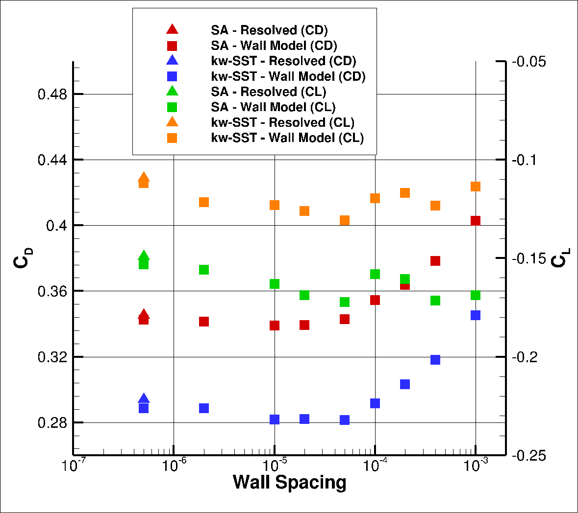
Fig. 116 Drag values for the Windsor case for a range of wall spacings for the Spalart-Allmaras and
The integrated loads show similar behaviour as for the Ahmed body case. At low wall spacings, both the predicted lift and drag coefficients start to decrease, when compared to wall-resolved simulations up to a wall spacing of 5e-05. As the wall spacing is increased further the lift convergence with wall spacing becomes non-monotonic and the drag increases. For both turbulence models, the best drag prediction agreement is obtained for a wall spacing of 2.5e-04, with the drag values being extremely close to the wall-resolved simulations. To examine these differences in greater detail, first the

Fig. 117 Y+ values along the centerline (y=0) of the Windsor body for wall-resolved (R) and wall-model simulations for the Spalart-Allmaras and
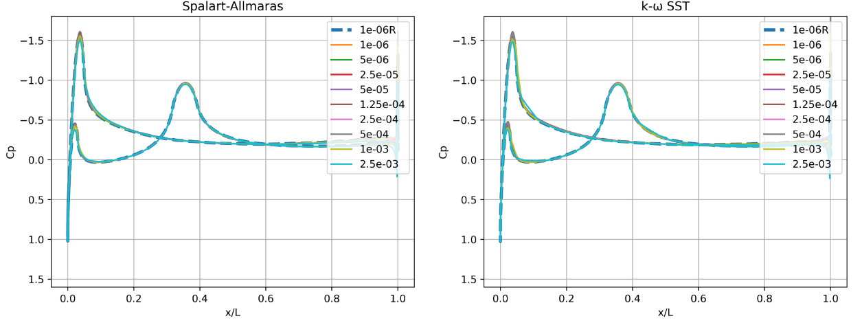
Fig. 118 Surface pressure predictions along the centerline (y=0) of the Windsor body for wall-resolved (R) and wall-model simulations for the Spalart-Allmaras and
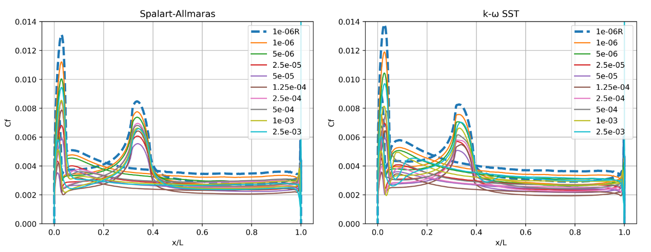
Fig. 119 Skin friction predictions along the centerline (y=0) of the Windsor body for wall-resolved (R) and wall-model simulations for the Spalart-Allmaras and
The
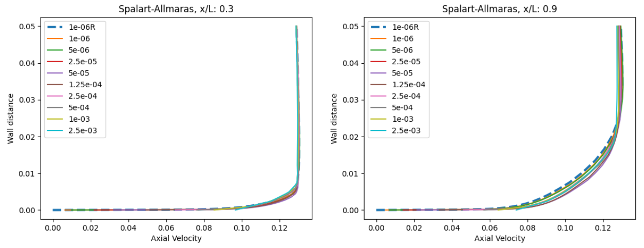
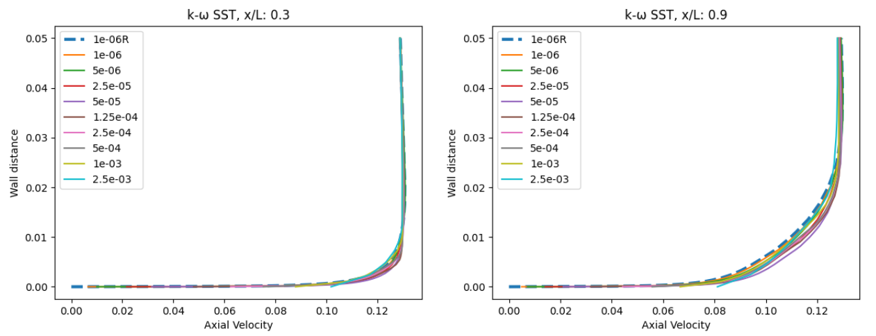
Fig. 120 Velocity profile predictions for the Windsor body case for wall-resolved (R) and wall-model simulations at two locations along the centerline (y=0) for the Spalart-Allmaras and
The velocity profiles show a high degree of consistency between the wall-resolved and wall-model simulations. The minor differences are slightly larger at x/L=0.9 than at x/L=0.3, however, the excellent agreement across all wall spacings is very promising. There is a minor difference in the wall velocity predicted by the two different turbulent models. Finally, the flowfield streamline patterns are extracted from the solutions on the symmetry plane, shown in Fig. 121.
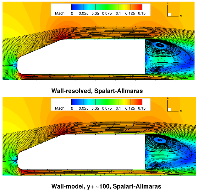

Fig. 121 Flowfield predictions along the centerline (y=0) for the Windsor body case for wall-resolved (R) and wall-model (at ~100
Similarly as for the Ahmed body case, the flowfields are very consistent between wall-resolved and wall-modelled simulations. The acceleration over the top of the car and between the car underbody and floor is well captured with similar flow patterns in the car wake. Here, slightly different recirculation patterns are predicted when comparing the Spalart-Allmaras and
Conclusions#
This case study leads to the following recommendations and conclusions for investigations that include wall modeling:
The wall model has been validated against wall-resolved simulations for a number of test cases including aerospace and automotive applications, leading to very good agreement in the integrated loads predictions.
No robustness issues were found with the wall model even at very high CFL numbers, higher than would be typically used for wall-resolved simulations, although the model robustness will reduce at very high
The best agreement in integrated loads was obtained for
The use of the wall model typically has minor impact on the surface pressure prediction, but will lead to an error on the skin friction distributions. Generally, however, the skin friction trends are well captured based on the examined cases.
The optimal compromise between computational cost and accuracy are target
The wall model does not perform well under the presence of strong pressure gradients, which is the case in aerospace applications near stall. The current wall model formulation does not account for pressure gradient effects. Therefore, for such flows, wall-resolved simulations are recommended.