2D NACA 4412 Airfoil Trailing Edge Separation

Introduction

The main purpose of this case is validation of the Flow360 solver against experimental data and other CFD solvers, primarily CFL3D. Three different turbulence models are evaluated for this case: SA, SA-RC and k- ω SSTm. The case is part of the NASA Turbulence Modelling Website and has also been evaluated by other CFD solvers such as OVERFLOW in Jespersen et al . The experimental data includes surface pressure data as well as velocity profiles near the trailing edge of the airfoil. While primarily being a validation case for capturing the trailing edge separation, certain model implementation verification can be performed by comparing the results with other CFD codes.

Simulation setup

A single C-Topology grid is used, available at the NACA4412 case grid download page of the TMR website. The second finest grid (897 by 257 points) is used to perform direct comparisons with CFL3D and FUN3D on the same grid. The grid used in Flow360 was modified for the names and number of boundaries, and is available here A detailed grid convergence study is not performed here. The grid far-view and near-view is shown in Fig. 31.

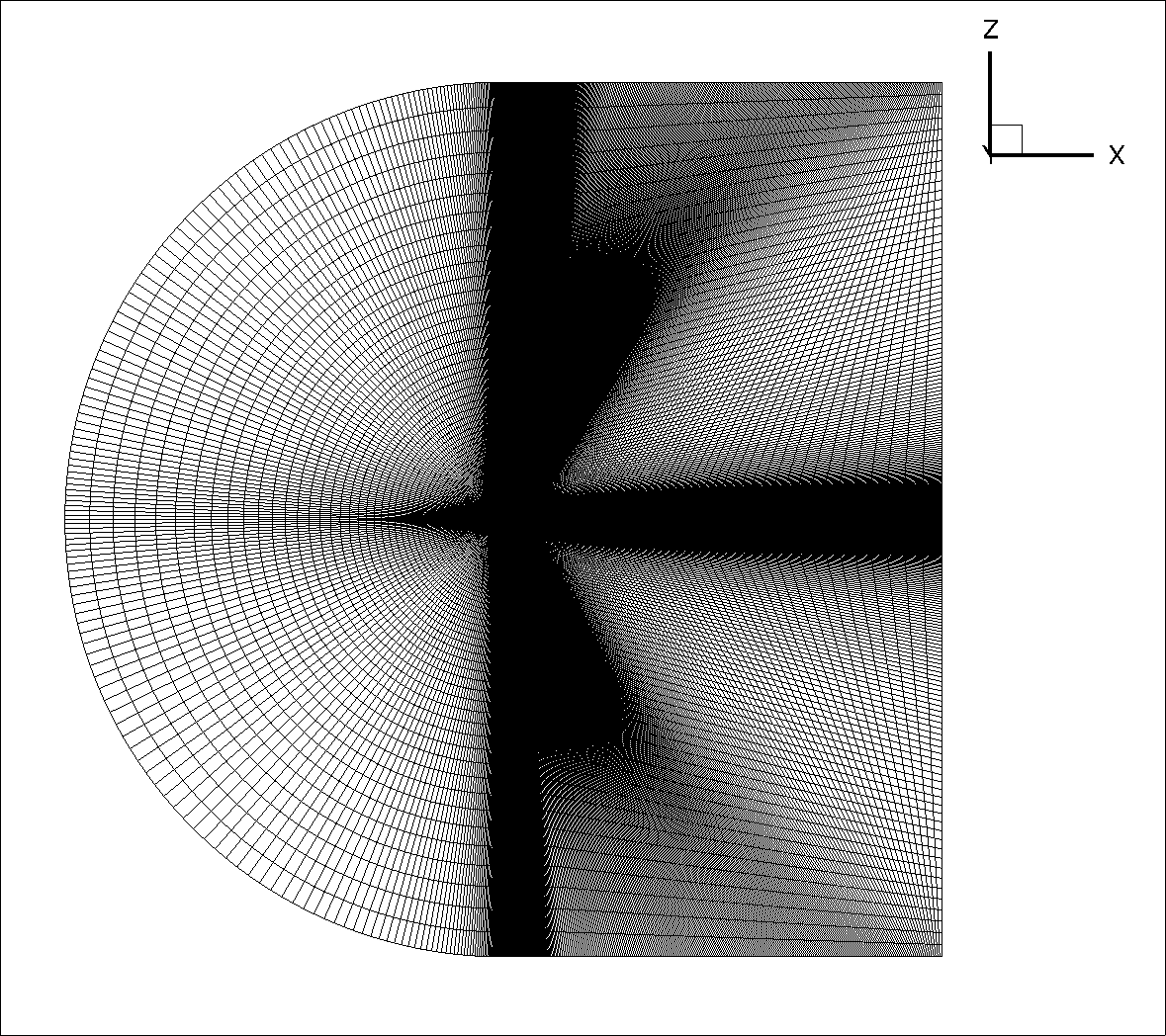
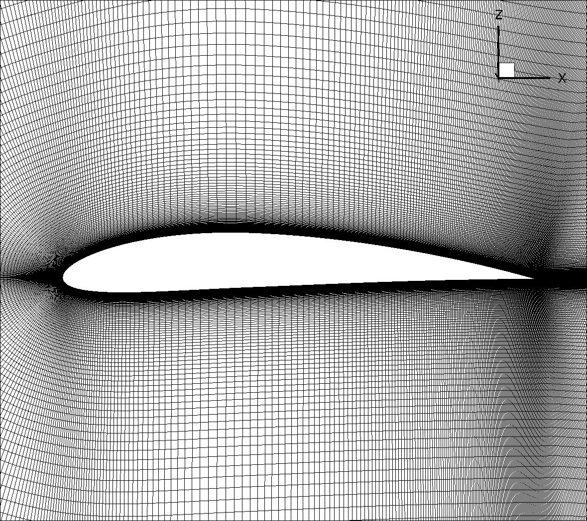
Fig. 31 Far-field and near-field views of the grid used for the NACA4412 trailing edge separation study.

A farfield Riemann boundary condition is used which is placed 100 chords away from the airfoil. The flow conditions were set to 1.52 million Reynolds number and a Mach number of 0.09. The study was performed for an angle of attack of 13.87 degrees. A reference temperature of 297.778K was used. Fully-turbulent calculations were performed with the ratio of the freestream value of the SA turbulence field variable (relative to laminar) set to 3, set in Flow360 as a turbulent viscosity ratio of 0.210438. For the k- ω SSTm calculations a turbulent viscosity ratio of 0.009 was used. Fig. 32 shows the case layout in detail, whereas the solver inputs are summarized in Table 6.

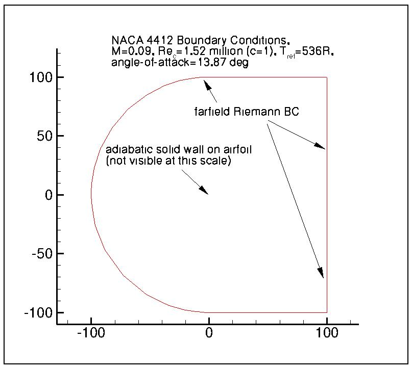
Fig. 32 Summary of case boundary conditions and conditions for the NACA4412 trailing edge separation study.

Table 6 Solver inputs for the NACA4412 trailing edge separation study.

Parameter	Value
Reynolds number	\(1.52 \times 10^6\)
Mach number	0.09
Reference temperature	297.778K
Angle of attack	\(13.87^o\)
Freestream turbulent viscosity ratio	0.210438 (SA), 0.009 (\(k-\omega\) SSTm)
CFL number	200

The simulations were performed using a CFL number of 200 ramped up over the initial 2000 iterations. To ensure deep convergence of the simulaitons, the CFL number was reduced to a value of 20, along with reducing the Jacobian update frequency from 4 to 1 towards the end of the simulations, although the impact on the integrated loads was minimal. For the majority of simulations, 1e-12 residual convergence was obtained for the flow residuals and 1e-10 for the turbulence residuals. The Flow360Mesh.json and Flow360.json files are provided for the SA model simulations (compatible with the modified NACA4412 grid for number of boundaries and boundary names).

Numerical Results

Firstly, the integrated are compared between Flow360, CFL3D, FUN3D, OVERFLOW for the SA, SA-RC and k- ω -SSTm turbulence models, shown in Table 7. Note the OVERFLOW code uses the baseline k- ω SST model, whereas the k- ω SSTm model is used by CFL3D, FUN3D and Flow360.

Table 7 Comparison of integrated loads between different CFD solvers for the NACA4412 aerofoil using the SA, SA-RC and k- ω -SSTm turbulence models.

Code	Turb. model	\(C_L\)	\(C_D\)	\(C_{Dp}\)	\(C_{Dv}\)
CFL3D	SA	1.7210	0.02861	0.02156	0.007042
FUN3D	SA	1.7170	0.02947	0.02246	0.007006
OVERFLOW	SA	1.7195	0.00309	\(-\)	\(-\)
Flow360	SA	1.7178	0.02905	0.022046	0.007008
CFL3D	SA-RC	1.7062	0.03000	0.02367	0.006325
FUN3D	SA-RC	1.7009	0.03087	0.02459	0.006289
Flow360	SA-RC	1.6980	0.03040	0.02408	0.006319
CFL3D	\(k-\omega\) SSTm	1.616	0.0311	0.0242	0.00687
FUN3D	\(k-\omega\) SSTm	1.615	0.0320	0.0252	0.00684
OVERFLOW	\(k-\omega\) SSTm	1.621	0.0321	\(-\)	\(-\)
Flow360	\(k-\omega\) SSTm	1.6225	0.03103	0.024194	0.006836

For the SA turbulence model, the Flow360 results agree very well with FUN3D integrated loads. The SA-RC model shows good agreement for the lift coefficient with FUN3D, whereas the drag coefficient is in between the CFL3D and FUN3D data. For the k- ω SSTm model, excellent agreement is also obtained with Flow360 integrated loads closer matching CFL3D data. In general, based on the integrated loads Flow360 shows excellent agreement with other CFD codes, as the differences between the different codes are similar as between other established CFD codes.

The surface pressure and skin friction coefficients are analysed next, and are compared with the CFL3D code and experimental data in Fig. 33 and Fig. 34

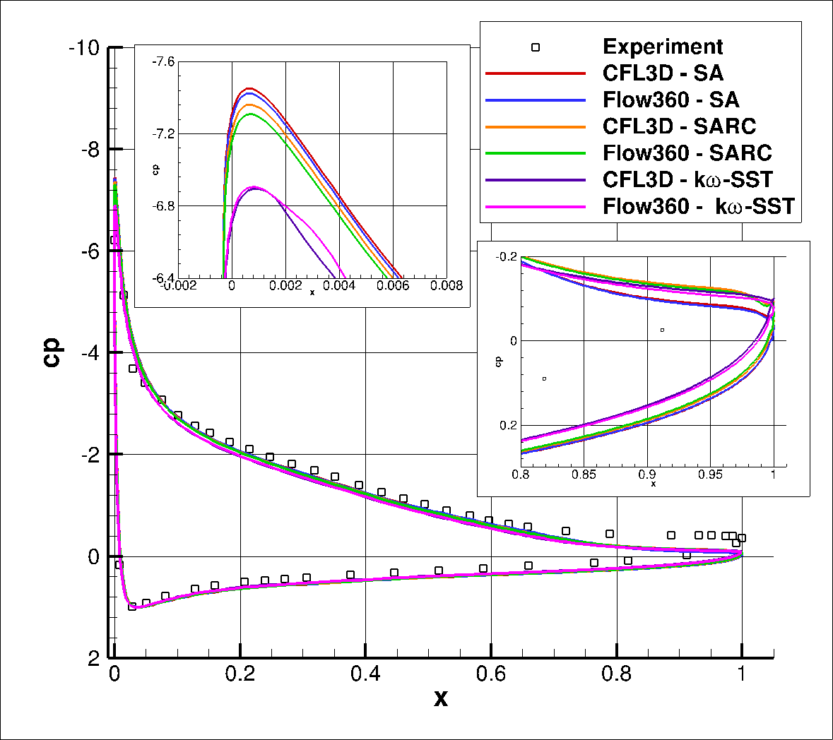
Fig. 33 Comparison of the surface pressure coefficients between Flow360 and CFL3D using three different turbulence models.

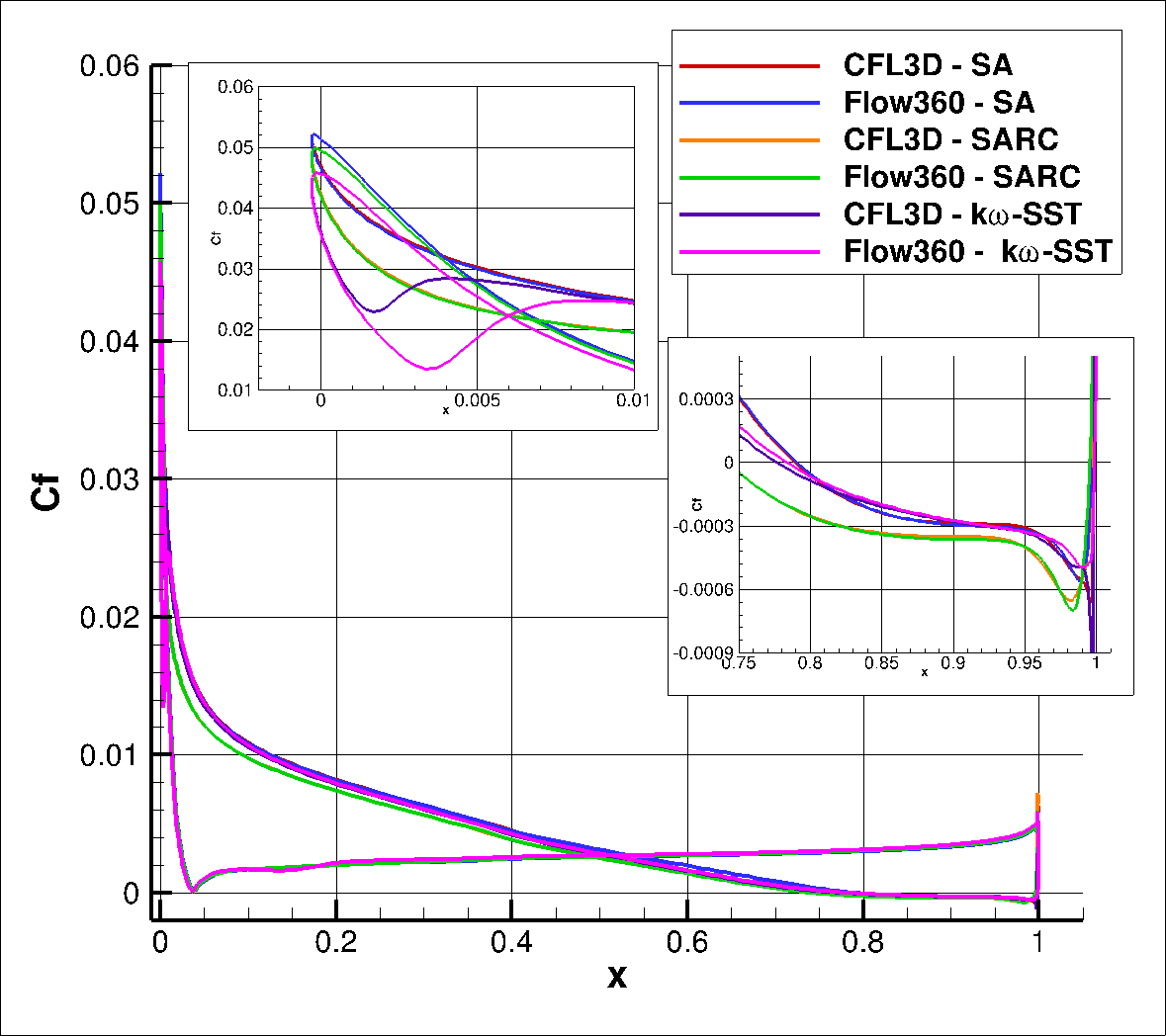
Fig. 34 Comparison of the skin friction coefficients between Flow360 and CFL3D using three different turbulence models.

Firstly, analysing the differences between Flow360 and CFL3D, excellent agreement is seen for the SA and SA-RC models in both the pressure coefficient and skin-friction coefficient chordwise distributions. Certain minor differences can been for the k- ω SSTm turbulence model near the leading edge, espeically for the skin friction coeffiicent, with good agreement in the trailing edge separation prediction. Comparing the difference turbulence models, the SA and SA-RC models lead to similar pressure distributions, with a slightly lower suction peak seen for the SA-RC model. The flow separates further upstream for the SA-RC model compared to the SA and k- ω SSTm turbulence models. The k- ω SSTm turbulence model predicts a much lower suction peak, but the skin friction profiles show similar behaviour to the SA model with only minor differences near the leading edge and trailing edge.

Further analysis is performed by comparing the velocity profiles including the turbulent shear stress at six locations along the airfoil chord with data from CFL3D and experiment. The data is normalized by a \(0.93 U_{ref}\) for the U and V velocities, and \(0.93^2 U_{ref}^2\) for the turbulent shear stress as indicated on the NASA Turbulence Modelling NACA4412 case website. The slice locations are at x/c = 0.6753, 0.7308, 0.7863, 0.8418, 08973 and 0.9528 shown in Fig. 35. The velocity profiles for the three turbulence models are compared in Fig. 36. The data was extracted using two line probes with uniformly spaced points in Tecplot (one finer line probe for the inner portion of the boundary layer and one coarser line probe for the outer portion). This was done, as the gradients were computed in Tecplot and using the direct CFD data leads to discontinuities in the turbulent shear stress profiles.

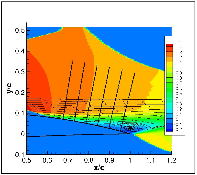
Fig. 35 Locations of the slices at which the velocity and turbulent shear stress profiles are compared.

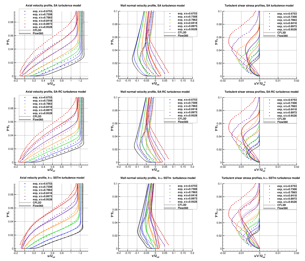
Fig. 36 Comparison of Velocity and turbulent shear stress profiles at six locations between experimental data, Flow360, and CFL3D for three turbulence models.

Firstly, comparing Flow360 and CFL3D results, excellent agreement can be seen for the U and V velocity profiles as well as the turbulent shear stress profiles for the SA and SARC turbulence models. The profiles obtained from both CFD codes are nearly identical. For the k- ω SSTm turbulence model, certain minor difference can be seen especially in the turbulence shear stress profiles, although the agreement is still reasonable. Similar differences were seen between CFL3D and OVERFLOW in Jespersen et al. Flow360 predicts a slightly higher V velocity at each chordwise location and reduced peak turbulence shear stress. Comparing the different turbulence models, the SA and SARC models lead to reduced boundary layer thickness and peak turbulent shear stress compared to experiment, although the SARC model shows an improvement over the SA model. The k- ω SSTm turbulence model leads to velocity profile predictions that are much closer to experimental data, although the turbulent shear stress magnitude is still undepredicted. Comparisons between Flow360 and CFL3D are also performed for the flow field solutions, shown in Fig. 37.

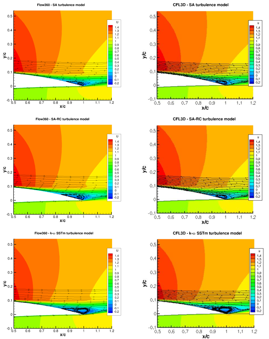
Fig. 37 Comparison of the flow field solutions between Flow360 and CFL3D for three turbulence models.

The flowfield solutions also show good agreement between Flow360 and CFL3D, with streamline differences attributed mainly due to different seeding locations between the two codes. The separation bubble grows in size when using the k- ω SSTm model when compared to the SA and SARC models predicted by both codes.

Overall, the results between Flow360, experimental data and other CFD codes show a high degree of consistency leading to further validation and verification of the Flow360 solver. The solver version release-22.2.3.0 was used throughout this study.