Scale-Resolving Simulations Past a Circular Cylinder

Introduction

The main purpose of this case study is the verification and validation of the scale-resolving techniques implemented in the Flow360 solver to represent turbulence. A Detached-Eddy Simulation is a three-dimensional unsteady solution based on a single turbulence model that functions as a sub-grid-scale model in a fine-grid region for a large-eddy simulation (LES) and as a Reynolds-averaged Navier-Stokes (RANS) model where the grid is not fine. Here, we are comparing the grid spacing with the thickness of the turbulent layer. It is possible for a DES grid to become excessively refined in some regions to capture a flow feature. In that case, the original DES length scale can become smaller than the boundary-layer thickness, which causes an early activation of the LES mode which is undesirable. This issue is known as “modeled-stress depletion” (MSD). A general approach to address MSD is to detect and shield the attached boundary layers and delay the activation of the LES mode even on grids where the DES length scale, which is proportional to the grid spacing, becomes smaller than the boundary-layer thickness. This approach was proposed by Spalart et al in 2006 as Delayed Detached-Eddy Simulation (DDES) (pure DES was introduced in 1997).

Turbulent flow contains a broad range of scales of length and time. The largest scales are related to the geometry and boundary conditions, while at the smallest length scales energy is dissipated by molecular viscosity. Simulations that capture all length scales of motion through a numerical solution of the Navier-Stokes (NS) equations are called direct numerical simulation (DNS) , which is computationally very expensive. The RANS approach solves equations averaged over time; however, RANS has been inaccurate when applied to flows with significant large-scale unsteadiness. The Large eddy simulation (LES) approach is an intermediate in computational complexity to address incompatibility of RANS in dealing with unsteady physics. It considers that transport of momentum and energy is mostly due to the unsteady features in the larger length scales being resolved in time and space and the effect of smaller length scales can be represented by using subgrid-scale (SGS) models. The implicit LES (ILES) relies on the mesh resolution and the stabilization of the algorithm, and doesn’t have an explicit SGS model.

The Roe scheme is an approximate Reimann solver based on a Godunov type scheme that solves a localized Reimann problem to calculate the flux. The low-dissipation Roe is a modification of the Roe scheme to consider low Mach number problems and to achieve lower numerical dissipation in the range of higher resolved wave numbers for the scale-resolving simulations. Both the standard and the low-dissipation schemes are considered for this validation study.

In this case study, DDES and ILES simulations are performed for the cross flow over an infinite span circular cylinder to validate smooth separation where it provides the opportunity to show its competitiveness with both RANS and LES. We considered simulations with laminar separation (LS) at a Reynolds number 20,000. A DDES simulation is attractive because of the known issue of “gray area” between RANS and LES regions. When a rapid new large-scale instability affects the turbulence, both pure LES and DDES are very reasonable, especially when the separation happens due to sharp edges. The cylinder is a more challenging and better test case for testing the “grey-area failures” as well as the accuracy in predicting smooth-body separation which depends on the Reynolds number, surface curvature, pressure gradients, and other aspects of the flow.

Simulation Setup

The circular cylinder test case is based on experimental tests at different Reynolds numbers at which the flow undergoes laminar and turbulent separations. Experimental results for cross flow over a circular cylinder can be found in Turbulence effect on crossflow around a circular cylinder at subcritical Reynolds numbers and Fluctuating lift on a circular cylinder: review and new measurements. For numerical results, one can refer to Detached-Eddy Simulations Past a Circular Cylinder and Large-Eddy Simulation of the Flow Over a Circular Cylinder at Reynolds Number 2 × 10⁴. The freestream Mach number is equal to 0.03 with a Reynolds number of 20,000.

The boundary conditions are shown in Fig. 160. In order to study the flow over a “2D” bluff-body, it is necessary to perform 3D simulations and consider the impact of the boundary condition in the third direction according to Travin et. al.

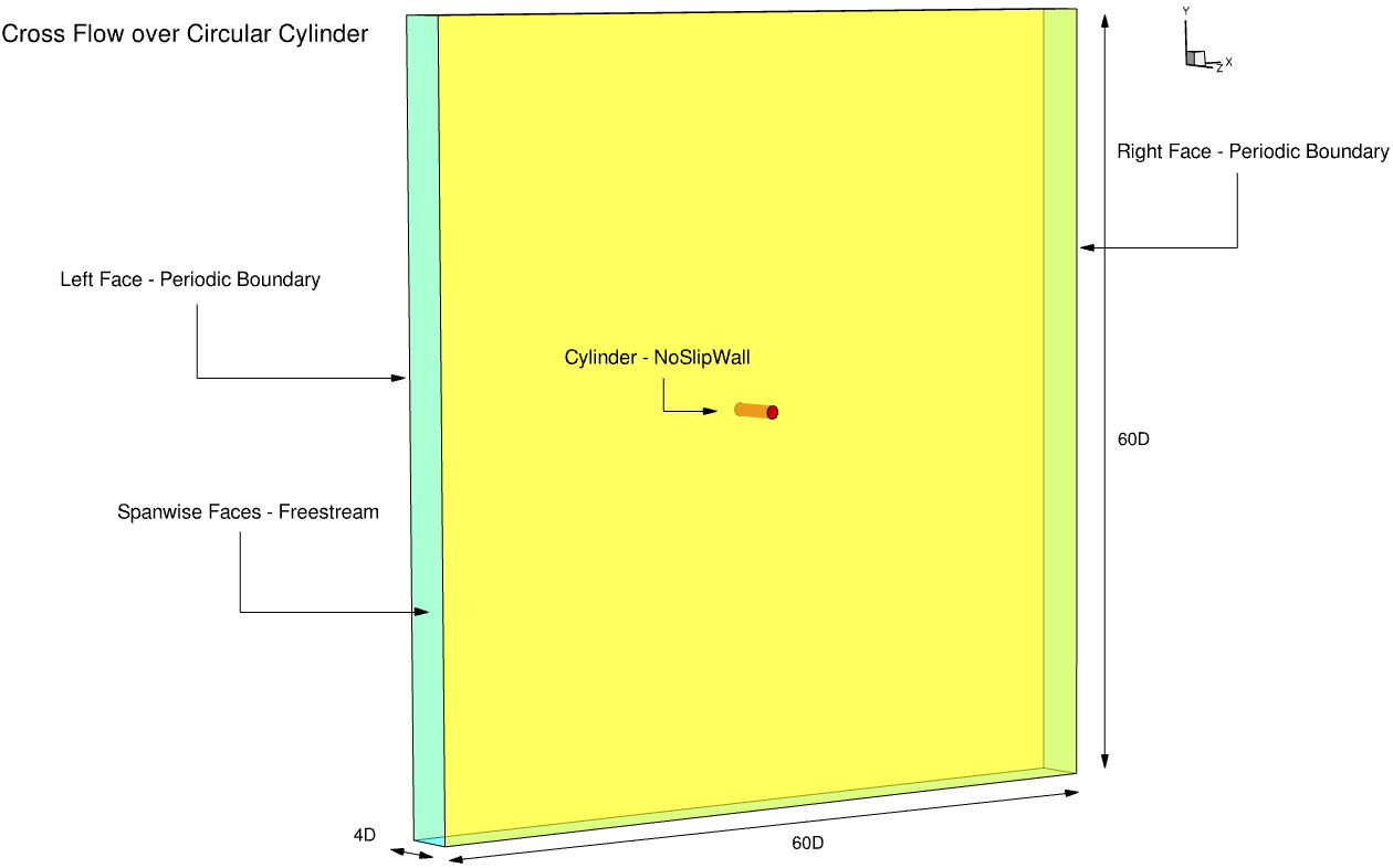
Fig. 160 Summary of boundary conditions and flow conditions for the cross flow over the circular cylinder case.

We used periodic boundary conditions and a spanwise length of \(L_{z}\) = 4 \(\times\) D to resolve the flow structure in comparison to the experiments. Because the freestream turbulence influences the instabilities in the separated shear layer, it is necessary to use periodicity. The entire domain has a dimension of 60D \(\times\) 60D \(\times\) 4D.

In general, we generated the grids with cubic hexahedron cells in the region away from the cylinder surface and sizing them according to the desired mesh resolution. It is recommended to refine the grid in all directions simultaneously. For the grid refinement study, three grid levels are generated. The mesh node statistics for the three mesh levels are presented in Table 31 with the meshes shown in Fig. 161.

For this case study, the grid refinement is a test for quality and sensitivity of solution accuracy to mesh resolution rather than a traditional convergence study. In the present work, we used 160 grid points in the coarse mesh, 225 points in the medium mesh and 320 in the fine mesh over the span length. For the coarse level, 500 mesh points; for the medium level, 703 points; and for the fine level, 1001 points, are distributed uniformly over the cylinder’s circumference. Number of mesh points in the x-y slice mesh outside the mesh boundary layer is shown in the table as “Wake”. The mesh resolving the boundary layer is built with hyperbolic extrusion and is thick enough to include the physical boundary layer.

Table 31 Grid levels for mesh refinement study.

Level	Circumferential	Spanwise	Boundary Layer	Wake	Total
Level 1	500	160	500×46	52026	11924160
Level 2	703	225	703×46	79906	25096725
Level 3	1000	320	1001×57	77739	42796480

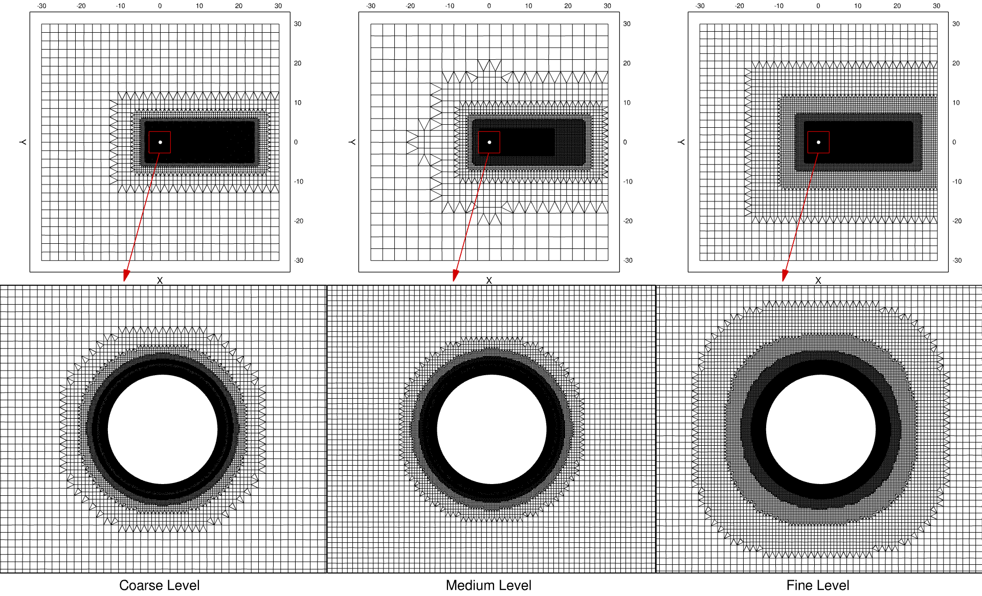
Fig. 161 Three grid levels generated for the cross flow over the cylinder.

For an unsteady simulation, the turbulent wake is considered as fully established after a duration of \(T \cdot U_{\infty}/D\) = 350 by Lysenko et. al, where T is the period, U is the freestream velocity and \(T =1/f\). The frequency of the vortex sheddings can be obtained by \(St=\frac{f \cdot D}{U_{\infty}}\). The time step size is decreased in three phases in order to establish the unsteady solution after 35 vortex sheddings. Afterwards, the solution is restarted with a smaller fixed time step size for a further 20 vortex sheddings. Gradually decreasing the time step size helps to quickly develop the solution for the initial 35 vortex sheddings. Moreover, time-step refinement helps to reduce the sources of numerical errors. In this case, the initial time step size of 0.54 is used. Then it is reduced to 0.35 and eventually to 0.14. All the time step sizes are non-dimensionalized using standard Flow360 conventions. For a quantitative validation of the present simulation, the solution is sampled over the last \(N_{vp}\) = 20 shedding cycles.

If the ILES simulation with the low-dissipation scheme is unstable, a smaller time-step size with a fixed, large CFL values can be used. For this case, the CFL number is fixed at 100,000. The low-dissipation factor can be adjusted to reduce the dissipation of the numerical scheme.

Grid Refinement Study

Results of the grid refinement study are presented in Table 32. The averaging operator is shown by \(\langle \rangle\). In this table, results on three grid levels for the time-averaged drag coefficient, root mean square of the lift coefficient \(\langle C_{l}\rangle\), Strouhal number \(\langle S_{t}\rangle\), and separation angle are presented. The results for the fine grid match the results reported in literature for this Reynolds number accurately. Based on the experimental results for Re = \(2 \times 10^{4}\), the root mean square of the lift coefficient \(C^{\prime}_{l}\) varies between 0.42 and 0.63. The experimental and numerical results in literature also assess \(\langle C_{d}\rangle\) = 1.2. The Strouhal number measured from the experiment is \(St_{exp}\) = 0.19 and the separation angle is \(\theta_{sep}\) = 78 °. A summary of experimental and numerical results at this Reynolds number can be found in Lysenko et. al. For the simulations results presented in Table 32, the Strouhal number is determined from FFT of the \(C_{l}\) time signal. The LDRoe scheme shows better agreement with experiment on medium mesh in comparison to the Roe scheme.

Table 32 Grid refinement study for ILES simulations with Roe and LDRoe schemes.

Grid	Method	Numerical Scheme	⟨Cd ⟩	RMS Cl	St	⟨θsep⟩
Level 1 (coarse)	ILES	Roe	1.3712	0.7044	0.19	84.7°
Level 1 (coarse)	ILES	LDRoe	1.2032	0.4528	0.2	82°
Level 2 (medium)	ILES	Roe	1.1458	0.3101	0.2	83.5°
Level 2 (medium)	ILES	LDRoe	1.1989	0.4517	0.2	83.1°
Level 3 (fine)	ILES	Roe	1.1965	0.4242	0.19	81.9°
Level 3 (fine)	ILES	LDRoe	1.1932	0.4809	0.19	82°
Experiment	‒	‒	1.2	0.42	0.19	78°

The time-averaged pressure coefficient over the mid section is plotted in Fig. 162 for three mesh levels. For both ILES simulations with the Roe and LDRoe schemes, the pressure coefficient for the fine mesh matches the experimental results reported by Norberg with a high degree of accuracy. However, with the Roe numerical scheme, the predictions using the coarse and medium meshes, follow the trends for the averaged pressure coefficient but they both are inaccurate after the separation point along the downstream face of the cylinder. On the contrary, with the low-dissipation numerical scheme, the results for the coarse and medium meshes are very close to the results on the fine mesh. This indicates that with the low-dissipation scheme on coarser mesh levels, more accurate results are achievable and the scheme is less dependent on mesh resolution or degrees of freedom.

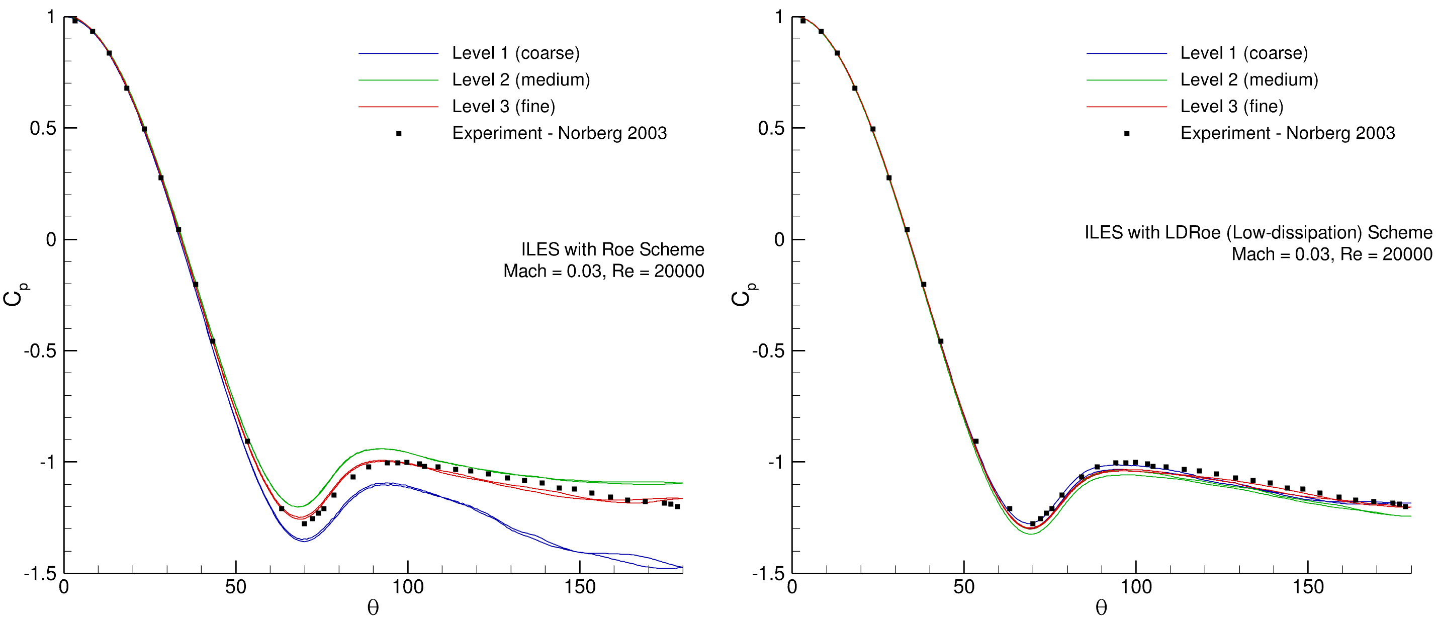
Fig. 162 Pressure coefficient comparison for three grid levels. Level 3 fine mesh, 43M nodes (red). Level 2 medium mesh, 24M nodes (green). Level 1 coarse mesh, 7.5M nodes (blue).

The time-averaged drag (\(C_{d}\)) and root-mean-square lift (\(C_{l}\)) coefficients are shown in Fig. 163 against grid convergence index (GCI). For both numerical schemes, the ILES simulations with the low-dissipation scheme are converging faster in comparison with the Roe scheme with increasing mesh resolution and showing asymptotic behavior.

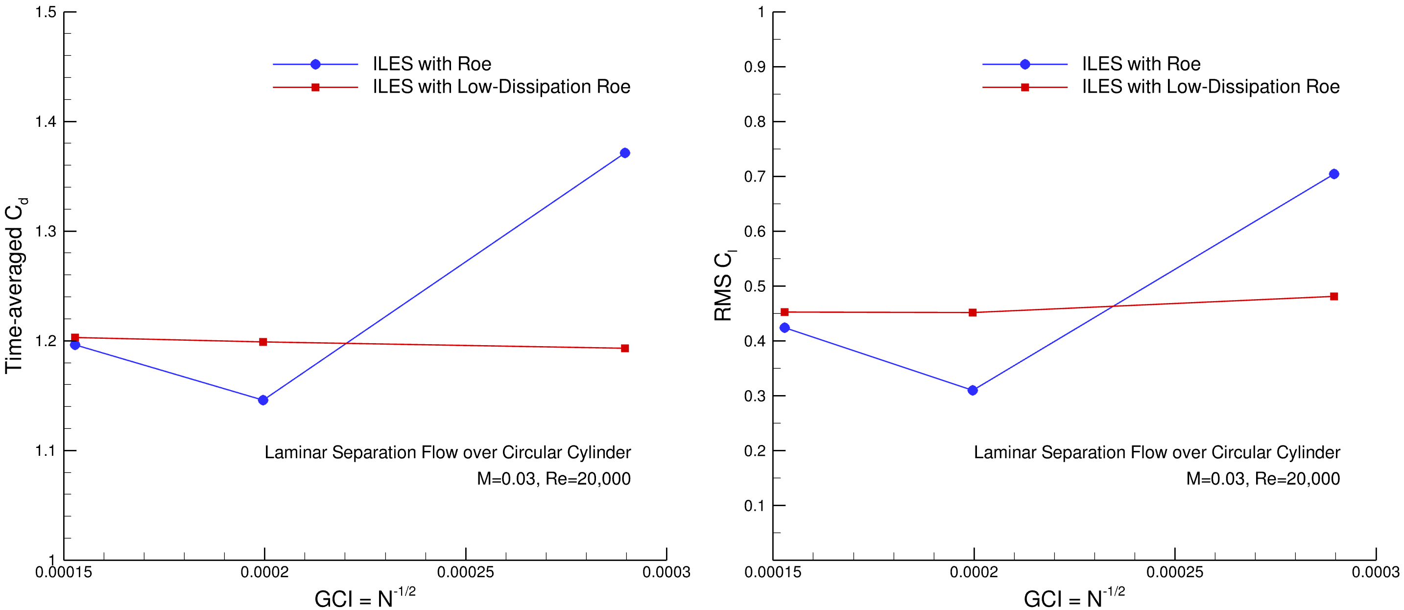
Fig. 163 Grid convergence figure for the time-averaged drag (\(C_{d}\)) and root-mean-square lift (\(C_{l}\)) coefficients on three grid levels for the cross flow over the cylinder.

Time-Dependent Flow Field Results

First, the loading time-histories are examined to investigate the impact of the numerical scheme on the load oscillation magnitudes and shedding cycle behavior. The time histories of aerodynamic coefficients for different methods are compared in Fig. 164. It shows the time histories of the lift (\(C_{l}\)) and drag (\(C_{d}\)) coefficients for a period of \(\approx\) 20 vortex shedding cycles for four simulations on the fine mesh. In all figures, an initial transient of length 35 was removed. The figures show that removing of 10 more cycles for DDES-SA simulations and for simulations with the low-dissipation scheme would have been desirable. All sub-figures show strong modulations of the shedding phenomenon. A higher drag is found with larger lift oscillation amplitude. The following drag coefficient comparison relate to this flow phenomenon. Compared to simulations with Roe scheme, low-dissipation schemes shows lower lift amplitude as shedding cycles are established.

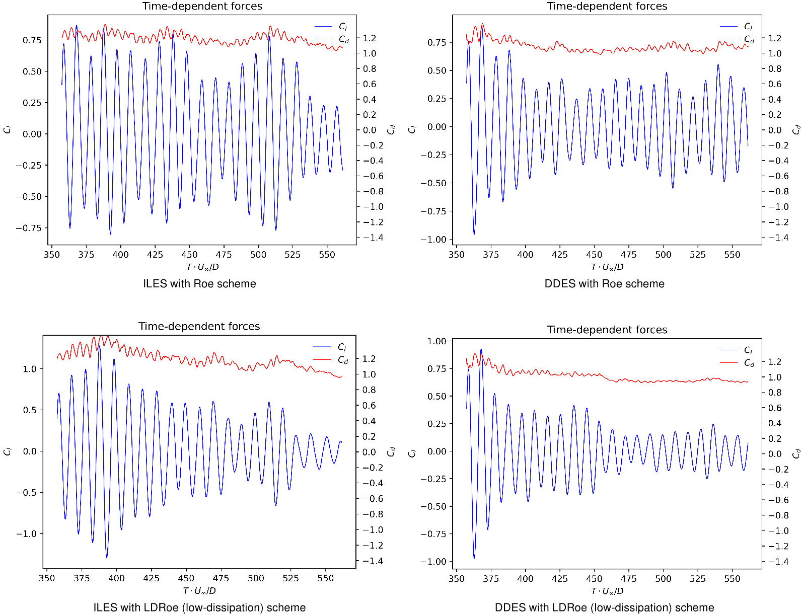
Fig. 164 Time history of the lift \(C_{l}\) and drag \(C_{d}\) coefficients (\(\approx\) 20 vortex shedding cycles) obtained from ILES and DDES simulations.

Fig. 165 shows the time histories of the aerodynamic coefficients for a the same period of \(\approx\) 20 vortex shedding cycles for the ILES and URANS simulations with the Roe scheme. Similar to previous simulations, an initial transient of length 35 shedding cycles is removed. The modulations of the shedding phenomenon is present in both. However, the Unsteady RANS simulation doesn’t show any change over the coarse of time in comparison to the ILES simulation.

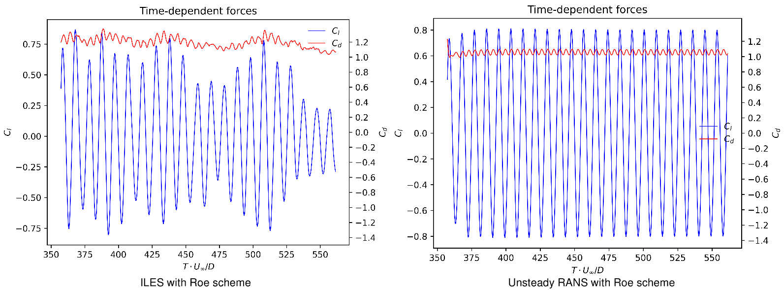
Fig. 165 Time history of the lift \(C_{l}\) and drag \(C_{d}\) coefficients (\(\approx\) 20 vortex shedding cycles) obtained from ILES and URANS simulations.

The iso-surface of Q-criterion is shown in Fig. 166 to clearly demonstrate the three dimensionality of the solutions. The iso-surface figures for all simulations shows the vortex core that starts from the shear layer on the upper and lower surface of the cylinder. The ILES simulations are capturing the much small vortices near the cylinder after the separation. Both simulations with low-dissipation schemes either ILES or DDES shows finer vortex features.

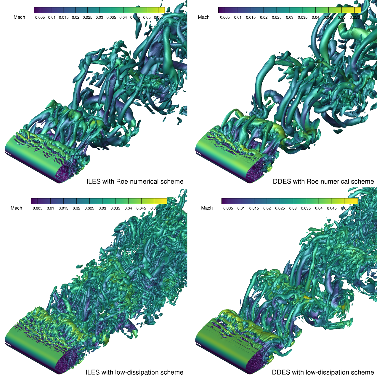
Fig. 166 Iso-surfaces obtained from ILES and DDES simulations for the flow over a circular cylinder at Re= \(2 \times 10^{4}\)

From the side view, the iso-surface of Q-criterion is shown in Fig. 167 that reveals a dominant 2D von Karman vortex-shedding mode in all simulations. The ILES and DDES simulations with the Roe scheme show very similar vortex features in the wake. The ILES simulation is slightly better in capturing flow features. The ILES and DDES simulations with the low-dissipation scheme captures finer flow features in the wake and near the cylinder after the separation. The ILES simulation with the low-dissipation scheme shows finer vortex structures in comparison to others.

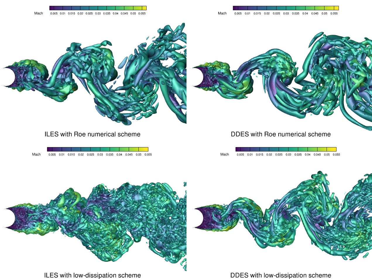
Fig. 167 Iso-surfaces obtained from ILES and DDES simulations for the flow over a circular cylinder at Re= \(2 \times 10^{4}\)

In order to make a comparison between the different methods, the iso-surface of Q-criterion for an unsteady RANS, DDES based on the SA turbulence model, ILES with the Roe scheme and ILES with the low-dissipation Roe scheme is shown in Fig. 168. This comparison shows that by adding to the fidelity of an unsteady simulation, more complete flow features can be captured. The DDES versus ILES with the Roe scheme primarily differ in the region of boundary layer separation. The ILES with the low-dissipation Roe scheme resolves the downstream vortex structures significantly better than other methods, improving the accuracy and reliability.

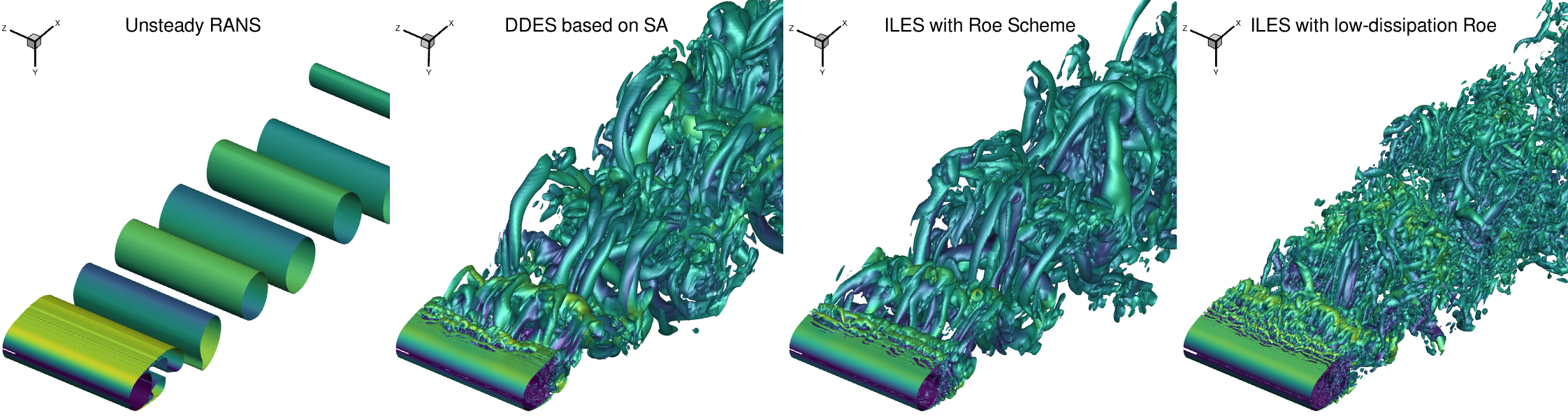
Fig. 168 Iso-surfaces obtained from unsteady RANS, DDES, ILES with the Roe and low-dissipation Roe simulations for the flow over a circular cylinder at Re= \(2 \times 10^{4}\)

The instantaneous contours of vorticity magnitude on the x-y plane for the ILES and DDES simulations are shown in Fig. 169. All instantaneous frames are at \(T \cdot U_{\infty}/D\) = 550. They all are on the fine mesh. The Roe scheme does not capture the small flow features in the recirculation region, while flow features are captured very well in this region and near the laminar boundary layer separation with the low-dissipation scheme.

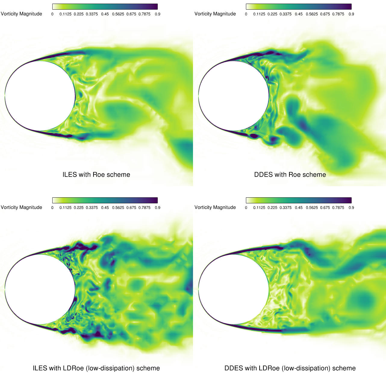
Fig. 169 Vorticity magnitude contours in the x-y plane obtained from ILES and DDES simulations for the flow over a circular cylinder at Re= \(2 \times 10^{4}\)

Time-Averaged Flow Field Results

In this section, time-averaged flow field results are compared against experiment and numerical results. It shows how well different methods predict time-averaged flow quantities for the cross flow over the circular cylinder with unsteady flow behavior. Fig. 164 shows the time-averaged streamlines in the x-y plane for the ILES and DDES simulations. Besides the main recirculation bubble, vortices attached to the downstream surface of the cylinder are present in all the results. The existence of the small secondary vortices at the back side of the cylinder is confirmed by experimental results by Lysenko et. al. This shows that several separation angles beside the primary separation exist. The primary separation based on the experimental results is at \(\langle \theta_{s1} \rangle=\) 78 ° and the secondary separation is at \(\langle \theta_{s2} \rangle=\) 108 °. The DDES simulations show a greater recirculation length in the wake region. The recirculation length \(\langle L_{r} \rangle\) indicates the distance between the base of the cylinder and the sign change of the centerline mean stream-wise velocity. Unfortunately, there is no experimental results for the recirculation length at this Reynolds number.

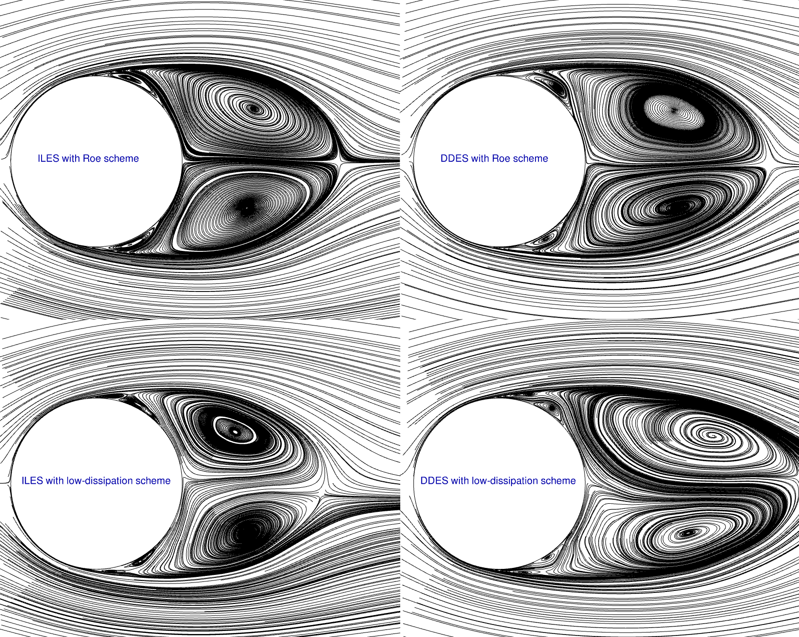
Fig. 170 Time-averaged streamline in the x-y plane obtained from ILES and DDES simulations for the flow over a circular cylinder at Re= \(2 \times 10^{4}\)

The time-averaged pressure coefficient over the cylinder slice in the x-y plane is shown in Fig. 171. On the left, results for the ILES simulation are shown and match well with the experimental results provided by Norberg at Re= \(2 \times 10^{4}\). The ILES simulation with the low-dissipation scheme leads to slightly better agreement between \(\langle \theta \rangle=\) 78 ° and \(\langle \theta \rangle=\) 100 °. On the right, results for the DDES simulations are presented. The result for the DDES simulation with the Roe scheme is closer than the LDRoe predictions to the experiment in the backward side of the cylinder. The disagreement between the ILES and DDES simulations for the time-averaged pressure coefficients indicate the impact of laminar separation at this Reynolds number. For the time-averaged pressure coefficient, better correlation is expected when turbulent separation is considered.

The mean base suction coefficient \(\langle C_{p,b} \rangle\) is determined as the mean pressure coefficient on the cylinder’s surface at \(\langle \theta_{s1} \rangle=\) 180 °. It is strongly related to the mean drag coefficient. The calculated value of the mean base suction coefficient by ILES with the Roe scheme is \(\langle C_{p,b} \rangle=\) -1.16 and by ILES with LDRoe scheme is \(\langle C_{p,b} \rangle=\) -1.2. Both have good agreement with the experiment. The experimental value reported by Norberg is \(\langle C_{p,b} \rangle=\) -1.197. The calculated value by DDES with the Roe scheme is \(\langle C_{p,b} \rangle=\) -1.06 and by DDES with LDRoe scheme is \(\langle C_{p,b} \rangle=\) -0.962, which doesn’t show good agreement with the experiment in comparison to ILES simulations.

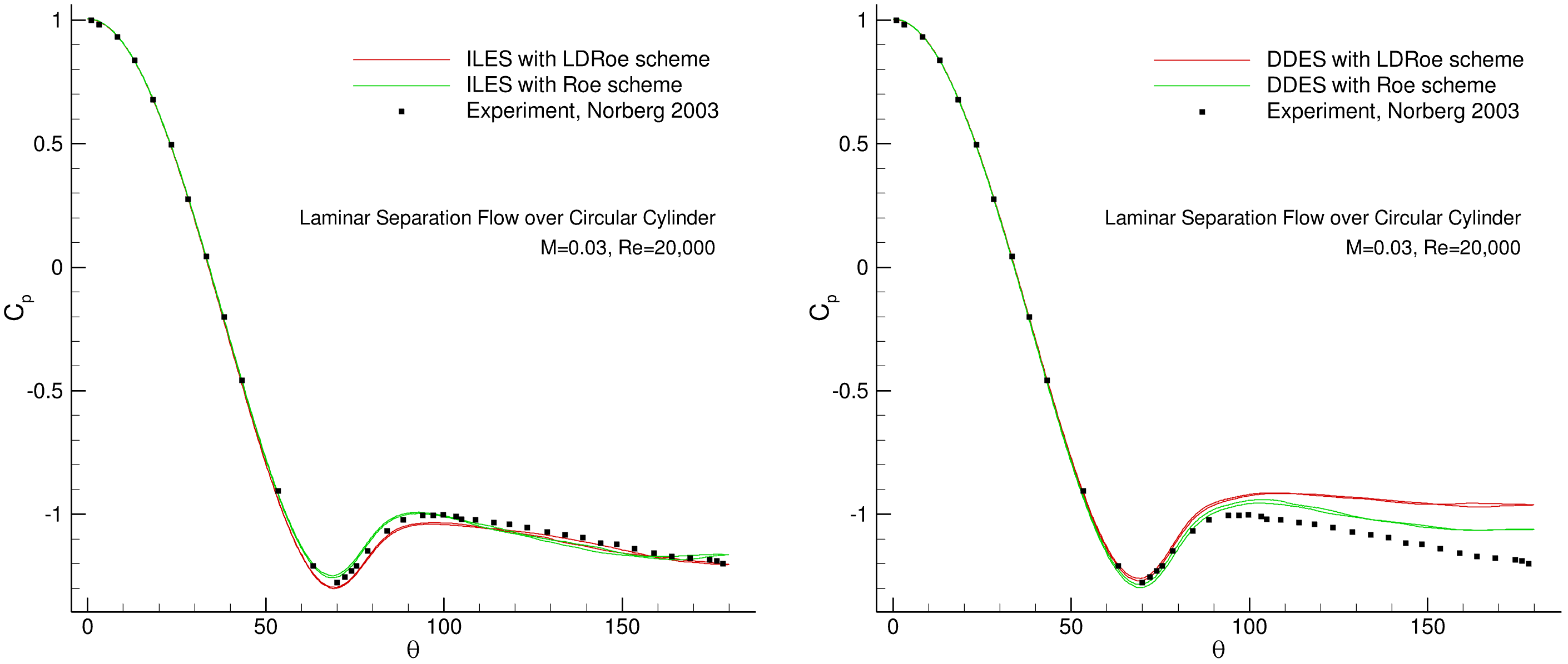
Fig. 171 Time-averaged pressure coefficient \(C_{p}\) obtained from ILES and DDES simulations for the flow over a circular cylinder at Re= \(2 \times 10^{4}\)

To compare the flow separation, the time-averaged skin-friction coefficients are shown in Fig. 172. Both ILES and DDES simulations with the Roe and LDRoe schemes have good agreement. The primary separation angle is \(\langle \theta \rangle=\) 78 ° based on the experimental results provided by Norberg. The separation angle for the ILES simulation with the Roe scheme is 81 ° and with the LDRoe scheme is 82 ° that both are in agreement with the experimental result. For the DDES simulations, the separation angles are also similar. This indicates both ILES and DDES methods and both Roe schemes on the fine mesh are closely predicting the expected primary separation angle.

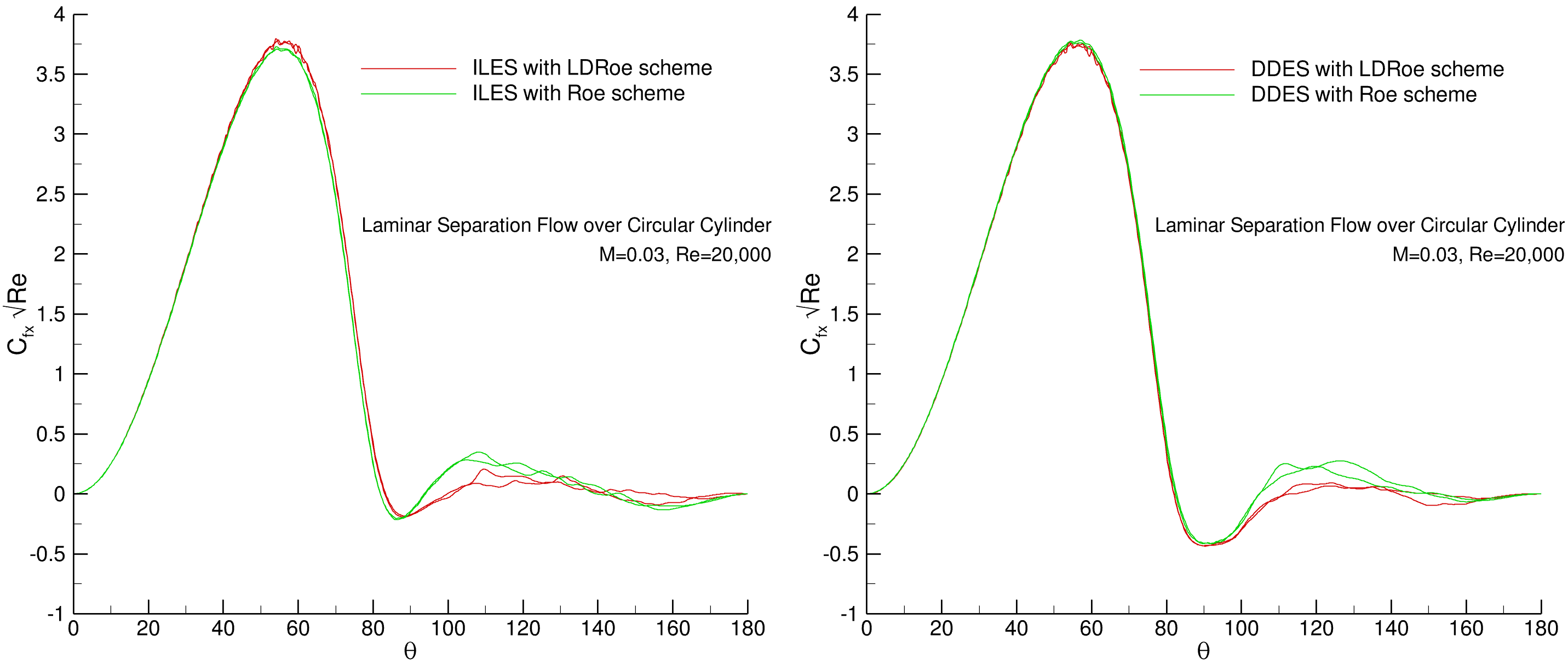
Fig. 172 Time-averaged skin-friction coefficient \(C_{f}\) obtained from ILES and DDES simulations for the flow over a circular cylinder at Re= \(2 \times 10^{4}\)

For a RANS, unsteady RANS, DDES and ILES simulations, time-averaged pressure \(C_{p}\) and skin-friction \(C_{f}\) coefficients are compared in Fig. 173 to make a comparison between different CFD methods for the cross flow over the circular cylinder. The steady RANS is very far from the experiment because of unsteady flow behavior. The unsteady RANS fails to predict the flow near and after the separation because of not accurately capturing the instabilities in the separated shear layer. The DDES simulation is close to experiment and the ILES simulation matches almost exactly with the experiment. Meanwhile, time-averaged quantities for these simulations are compared in Table 33.

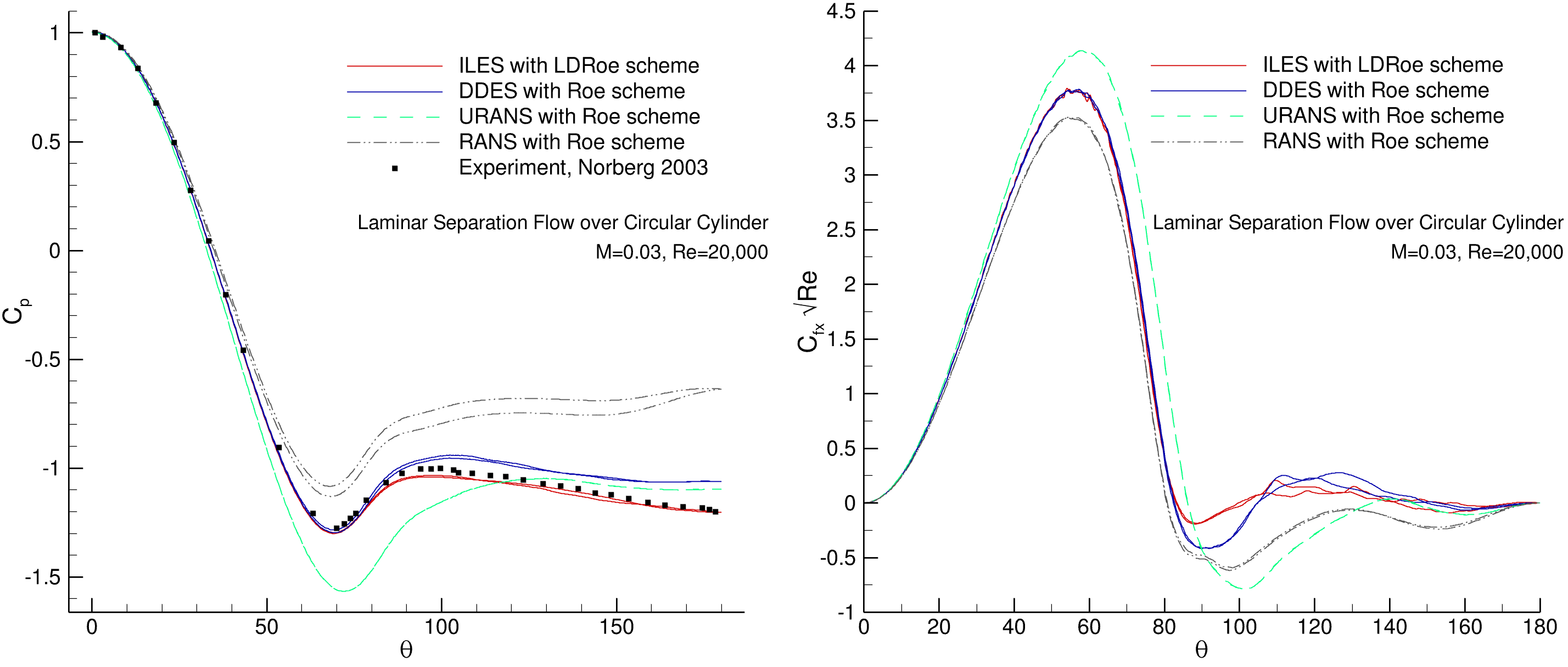
Fig. 173 Time-averaged pressure coefficient \(C_{p}\) and skin-friction coefficient \(C_{f}\) obtained from RANS, URANS, DDES and ILES simulations for the flow over a circular cylinder at Re= \(2 \times 10^{4}\)

Table 33 Wall-averaged quantities for the cross flow simulations over the circular cylinder with different methods on the fine mesh.

Method	Mesh	Scheme	⟨Cd ⟩	RMS Cl	St	⟨θsep⟩
RANS	Level 3 (fine)	Roe	0.8047	‒	‒	81°
URANS	Level 3 (fine)	Roe	1.0551	0.5617	0.219	88.5°
DDES	Level 3 (fine)	Roe	1.0898	0.3357	0.2	82°
ILES	Level 3 (fine)	Roe	1.1965	0.4242	0.19	81.9°
ILES	Level 3 (fine)	LDRoe	1.1932	0.4809	0.19	82°
Experiment	‒	‒	1.2	0.42	0.19	78°

The mean stream-wise velocity \(\langle u \rangle\) along the centerline is shown in Fig. 174. The minimum values of the mean stream-wise velocity predicted are \(\langle u_{min} \rangle/U_{\infty}=\) -0.27 for the ILES simulation with the low-dissipation scheme and \(\langle u_{min} \rangle/U_{\infty}=\) -0.24 for the DDES simulation with the low-dissipation scheme. For the ILES and DDES simulations with the Roe scheme, the \(\langle u_{min} \rangle/U_{\infty}\) respectively is -0.32 and -0.31.

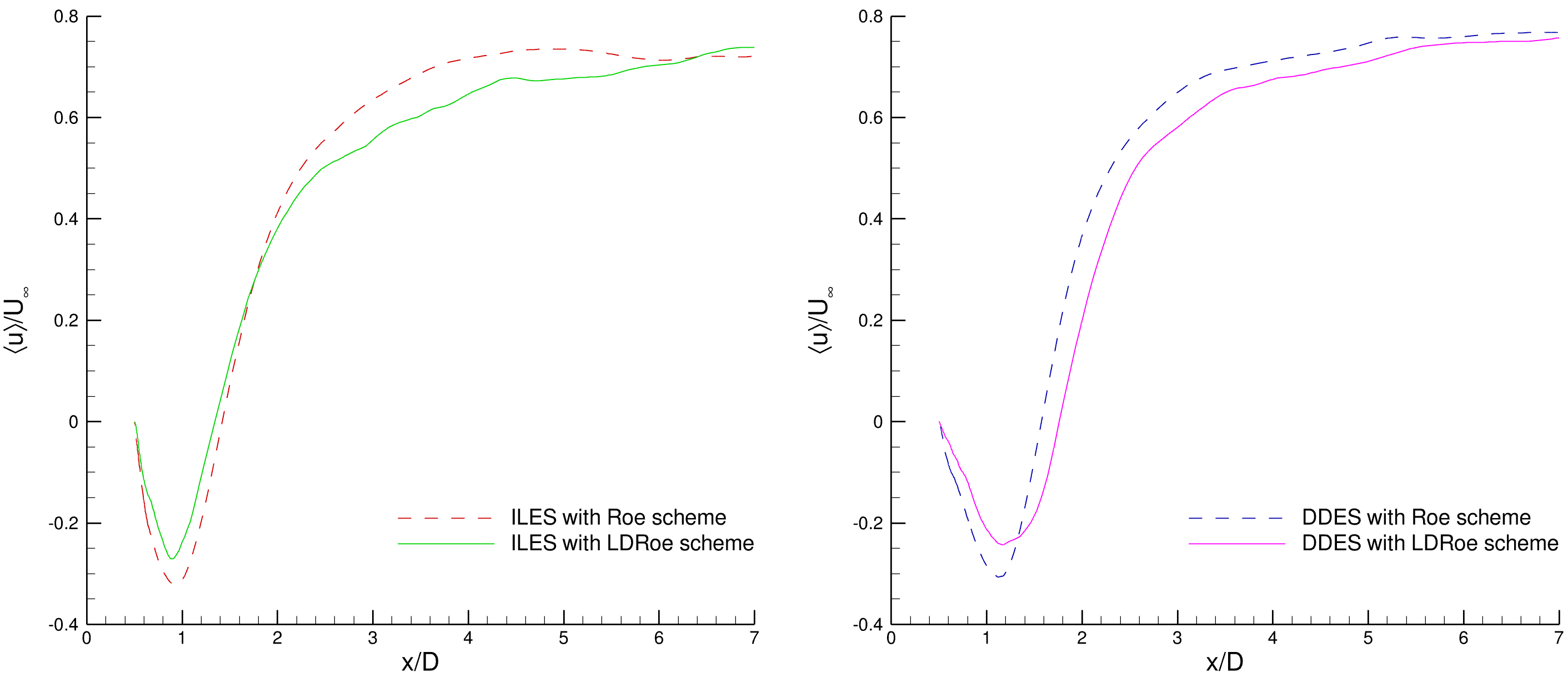
Fig. 174 Mean stream-wise velocity \(\langle u \rangle/U_{\infty}\) obtained from ILES and DDES simulations for the flow over a circular cylinder at Re= \(2 \times 10^{4}\)

An overview of the simulations and flow features from available experimental and numerical results are provided in Table 34. This table shows a comparison between the values obtained from the experiment and values obtained from different numerical methods. The results for the ILES simulations with both Roe and LDRoe schemes agree well with the experimental results. The ILES simulation with low-dissipation scheme performs better in predicting flow feature in the recirculation wake.

Table 34 Overview of the experimental, ILES and DDES works for the flow over a circular cylinder at Re= \(2 \times 10^{4}\).

Work	Method	Scheme	Mesh	Nvp	M	⟨Cd⟩	Cl’	St	˗⟨Cp⟩	⟨Lr⟩/D	˗⟨u⟩/U	⟨θsep⟩
Schewe⁽¹⁾	Exp					1.1	0.31	0.19				78°
Yokuda⁽²⁾	Exp					1.1			1.03
Norberg⁽³⁾	Exp						0.47	0.194	1.197			78°
Lim⁽⁴⁾	Exp					1.2		0.187	1.07
Salvatici⁽⁵⁾	LES	‒			0.1	0.98-1.17	0.38-0.46		0.96-1.12	0.77-0.86
Wornom⁽⁶⁾	LES	‒		30	0.1	1.27	0.6	0.19	1.09	0.8
Lysenko⁽⁷⁾	NSGS-I	‒		50	‒	1.3	0.75	0.2	1.2	0.44	0.11	88°
Lysenko⁽⁷⁾	TKE-I	‒		50	‒	1.32	0.64	0.2	1.05	0.64	0.19	86°
Lysenko⁽⁷⁾	NSGS	‒		75	0.2	1.35	0.65	0.17	1.13	0.57	0.16	87°
Lysenko⁽⁷⁾	TKE	‒		75	0.2	1.36	0.7	0.19	1.11	0.57	0.16	88°
Flow360	DDES	Roe	fine	20	0.03	1.0898	0.3357	0.2	1.06	1.08	0.31	82°
Flow360	DDES	LDRoe	fine	20	0.03	1.0128	0.2651	0.209	0.96	1.26	0.24	81°
Flow360	ILES	Roe	fine	20	0.03	1.1965	0.4242	0.19	1.16	0.91	0.32	81.9°
Flow360	ILES	LDRoe	fine	20	0.03	1.1932	0.4809	0.19	1.2	0.85	0.27	82°
Flow360	ILES	LDRoe	coarse	20	0.03	1.2092	0.4557	0.19	1.22	0.92	0.25	82°

Exp = Experiment

LES = Large Eddy Simulation

NSGS = No Subgrid-Scale

TKE = Turbulence Kinetic Energy

I = Incompressible

DDES = Delayed Detached-Eddy Simulation

ILES = Implicit Large Eddy Simulation

⁽¹⁾ Schewe G. On the force fluctuations acting on a circular cylinder in crossflow from subcritical up to transcritical Reynolds numbers. Journal of fluid mechanics. 1983 Aug;133:265-85.

⁽²⁾ Yokuda S, Ramaprian BR. The dynamics of flow around a cylinder at subcritical Reynolds numbers. Physics of Fluids A: Fluid Dynamics. 1990 May;2(5):784-91.

⁽³⁾ Norberg C. Fluctuating lift on a circular cylinder: review and new measurements. Journal of Fluids and Structures. 2003 Jan 1;17(1):57-96.

⁽⁴⁾ Lim HC, Lee SJ. Flow control of circular cylinders with longitudinal grooved surfaces. AIAA journal. 2002 Oct;40(10):2027-36.

⁽⁵⁾ Salvatici E, Salvetti MV. Large eddy simulations of the flow around a circular cylinder: effects of grid resolution and subgrid scale modeling. Wind and Structures. 2003 Nov 1;6(6):419-36.

⁽⁶⁾ Wornom S, Ouvrard H, Salvetti MV, Koobus B, Dervieux A. Variational multiscale large-eddy simulations of the flow past a circular cylinder: Reynolds number effects. Computers & Fluids. 2011 Aug 1;47(1):44-50.

⁽⁷⁾ Lysenko DA, Ertesvåg IS, Rian KE. Large-eddy simulation of the flow over a circular cylinder at Reynolds number 2×10 ⁴. Flow, turbulence and combustion. 2014 Mar;92:673-98.

Conclusions

This case study suggests the following recommendations for LES and DDES simulations:

• For 2D bluff-body flows, 3D simulations are necessary. The spanwise length is recommended to be at least \(3 \times D\) to resolve the flow structures observed in the experiment.

• For the modest subcritical regime, freestream turbulence influences the instabilities in the separated shear layer. For this reason, using periodicity is necessary and slipWall and symmetry should not be used.

• For simulations with a very low Mach number, it is necessary to have large enough domain to reduce the impact on the converged solution. Although larger domains need more physical steps for convergence.

• For bluff-body laminar separation flow:

  • Having enough mesh resolution in downstream wake is necessary for accurate results.

  • ILES simulations with the low-dissipation scheme provides the most accurate results compared to the experiment. In general, the low-dissipation scheme achieves more accurate results with less mesh resolution which indicates it is less dependent on the spatial degrees of freedom.

  • DDES simulations with the low-dissipation scheme are acceptable but are less accurate than ILES in the downstream side of the bluff-body. It is expected that for turbulent separation cases, DDES simulations will agree more closely with ILES simulations.

• For ILES simulations with the low-dissipation scheme, the simulation could be unstable, in that case a smaller time-step size with a fixed, large CFL values could help remedy this issue. Moreover, increasing the numerical low-dissipation factor helps to stabilize convergence. In this case study, a low-dissipation factor of 0.5 is used.

• The Flow360 solver is validated against experimental data and other scale-resolving simulations for laminar separation flow over a circular cylinder. Good agreement is found for time-dependent and time-averaged flow features and quantitative results.