Start here
Start here#
This is a basic Tidy3D script showing the FDTD simulation of a delectric cube in the presence of a point dipole.
[1]:
import numpy as np

# import the package and the web API
import tidy3d as td
import tidy3d.web as web
[21:36:34] WARNING  This version of Tidy3D was pip installed from the 'tidy3d-beta' repository on   __init__.py:103
                    PyPI. Future releases will be uploaded to the 'tidy3d' repository. From now on,
                    please use 'pip install tidy3d' instead.
INFO Using client version: 1.9.0rc1 __init__.py:121
[2]:
# set up parameters of simulation (length scales are micrometers)
grid_cells_per_wvl = 30
pml = td.PML()
sim_size = (4, 4, 4)
lambda0 = 1.0
freq0 = td.C_0 / lambda0
fwidth = freq0 / 10.0
run_time = 12.0 / fwidth

# create structure
dielectric = td.Medium.from_nk(n=2, k=0, freq=freq0)
square = td.Structure(
    geometry=td.Box(center=(0, 0, 0), size=(1.5, 1.5, 1.5)), medium=dielectric
)

# create source
source = td.UniformCurrentSource(
    center=(-1.5, 0, 0),
    size=(0, 0.4, 0.4),
    source_time=td.GaussianPulse(freq0=freq0, fwidth=fwidth),
    polarization="Ey",
)

# create monitor
monitor = td.FieldMonitor(
    fields=["Ex", "Ey", "Hz"],
    center=(0, 0, 0),
    size=(td.inf, td.inf, 0),
    freqs=[freq0],
    name="fields_on_plane",
)

# Initialize simulation
sim = td.Simulation(
    size=sim_size,
    grid_spec=td.GridSpec.auto(min_steps_per_wvl=grid_cells_per_wvl),
    structures=[square],
    sources=[source],
    monitors=[monitor],
    run_time=run_time,
    boundary_spec=td.BoundarySpec.all_sides(boundary=td.PML()),
)
[3]:
print(
    f"simulation grid is shaped {sim.grid.num_cells} for {int(np.prod(sim.grid.num_cells)/1e6)} million cells."
)
[21:36:35] INFO Auto meshing using wavelength 1.0000 defined from sources. grid_spec.py:510
simulation grid is shaped [192, 192, 192] for 7 million cells.
[4]:
# run the simulation, download the data.
data = web.run(sim, task_name="quickstart", path="data/data.hdf5")
[5]:
# see the log
print(data.log)
Simulation domain Nx, Ny, Nz: [192, 192, 192]
Applied symmetries: (0, 0, 0)
Number of computational grid points: 7.3014e+06.
Using subpixel averaging: True
Number of time steps: 1.2659e+04
Automatic shutoff factor: 1.00e-05
Time step (s): 3.1624e-17


Compute source modes time (s):     0.0472
Compute monitor modes time (s):    0.0024
Rest of setup time (s):            3.2856

Running solver for 12659 time steps...
- Time step    506 / time 1.60e-14s (  4 % done), field decay: 1.00e+00
- Time step    839 / time 2.65e-14s (  6 % done), field decay: 1.00e+00
- Time step   1012 / time 3.20e-14s (  8 % done), field decay: 1.00e+00
- Time step   1519 / time 4.80e-14s ( 12 % done), field decay: 1.44e-01
- Time step   2025 / time 6.40e-14s ( 16 % done), field decay: 3.23e-02
- Time step   2531 / time 8.00e-14s ( 20 % done), field decay: 1.37e-02
- Time step   3038 / time 9.61e-14s ( 24 % done), field decay: 6.90e-03
- Time step   3544 / time 1.12e-13s ( 28 % done), field decay: 3.30e-03
- Time step   4050 / time 1.28e-13s ( 32 % done), field decay: 2.38e-03
- Time step   4557 / time 1.44e-13s ( 36 % done), field decay: 1.63e-03
- Time step   5063 / time 1.60e-13s ( 40 % done), field decay: 1.20e-03
- Time step   5569 / time 1.76e-13s ( 44 % done), field decay: 7.23e-04
- Time step   6076 / time 1.92e-13s ( 48 % done), field decay: 4.98e-04
- Time step   6582 / time 2.08e-13s ( 52 % done), field decay: 2.31e-04
- Time step   7089 / time 2.24e-13s ( 56 % done), field decay: 1.57e-04
- Time step   7595 / time 2.40e-13s ( 60 % done), field decay: 6.76e-05
- Time step   8101 / time 2.56e-13s ( 64 % done), field decay: 7.59e-05
- Time step   8608 / time 2.72e-13s ( 68 % done), field decay: 4.44e-05
- Time step   9114 / time 2.88e-13s ( 72 % done), field decay: 6.20e-05
- Time step   9620 / time 3.04e-13s ( 76 % done), field decay: 2.67e-05
- Time step  10127 / time 3.20e-13s ( 80 % done), field decay: 3.19e-05
- Time step  10633 / time 3.36e-13s ( 84 % done), field decay: 1.45e-05
- Time step  11139 / time 3.52e-13s ( 88 % done), field decay: 2.07e-05
- Time step  11646 / time 3.68e-13s ( 92 % done), field decay: 5.97e-06
Field decay smaller than shutoff factor, exiting solver.

Solver time (s):                   7.5766
[6]:
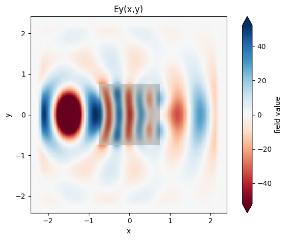
# plot the fields stored in the monitor
ax = data.plot_field("fields_on_plane", "Ey", z=0)
_ = ax.set_title("Ey(x,y)")
INFO Auto meshing using wavelength 1.0000 defined from sources. grid_spec.py:510
[ ]: