Tidy3D first walkthrough
Contents
Tidy3D first walkthrough#
Our first tutorial focuses on illustrating the basic setup, run, and analysis of a Tidy3D simulation. In this example, we will simulate a plane wave impinging on dielectric slab with a triangular pillar made of a lossy dielectric sitting on top. First, we import everything needed.
[1]:
# standard python imports
import numpy as np
import matplotlib.pyplot as plt
import h5py

# tidy3d imports
import tidy3d as td
from tidy3d import web
[00:00:26] WARNING  This version of Tidy3D was pip installed from the 'tidy3d-beta' repository on   __init__.py:103
                    PyPI. Future releases will be uploaded to the 'tidy3d' repository. From now on,
                    please use 'pip install tidy3d' instead.
INFO Using client version: 1.9.0rc1 __init__.py:121
First, we initialize some general simulation parameters. We note that the PML layers extend beyond the simulation domain, making the total simulation size larger - as opposed to some solvers in which the PML is covering part of the user-defined simulation domain.
[2]:
# Simulation domain size (in micron)
sim_size = [4, 4, 4]

# Central frequency and bandwidth of pulsed excitation, in Hz
freq0 = 2e14
fwidth = 1e13

# # pad the z direction (out of plane) with PML but leave it off x and y for periodic boundary conditions.
# boundary_spec=td.BoundarySpec.pml(x=False, y=False, z=True)

# apply a PML in all directions
boundary_spec = td.BoundarySpec.all_sides(boundary=td.PML())
The run time of a simulation depends a lot on whether there are any long-lived resonances. In our example here, there is no strong resonance. Thus, we do not need to run the simulation much longer than after the sources have decayed. We thus set the run time based on the source bandwidth.
[3]:
# Total time to run in seconds
run_time = 2 / fwidth
Structures and materials#
Next, we initialize the simulated structure. The structure consists of two Structure objects. Each object consists of a Geometry and a Medium to define the spatial extent and material properties, respectively. Note that the size of any object (structure, source, or monitor) can extend beyond the simulation domain, and is truncated at the edges of that domain.
Note: For best results, structures that intersect with the PML or simulation edges should extend extend all the way through. In many such cases, an “infinite” size td.inf can be used to define the size along that dimension.
[4]:
# Lossless dielectric specified directly using relative permittivity
material1 = td.Medium(permittivity=6.0)

# Lossy dielectric defined from the real and imaginary part of the refractive index
material2 = td.Medium.from_nk(n=1.5, k=0.0, freq=freq0)
# material2 = td.Medium(permittivity=2.)


# Rectangular slab, extending infinitely in x and y with medium `material1`
box = td.Structure(
    geometry=td.Box(center=[0, 0, 0], size=[td.inf, td.inf, 1]), medium=material1
)

# Triangle in the xy-plane with a finite extent in z
equi_tri_verts = [[-1 / 2, -1 / 4], [1 / 2, -1 / 4], [0, np.sqrt(3) / 2 - 1 / 4]]

poly = td.Structure(
    geometry=td.PolySlab(
        vertices=(2 * np.array(equi_tri_verts)).tolist(),
        # vertices=equi_tri_verts,
        slab_bounds=(0.5, 1.0),
        axis=2,
    ),
    medium=material2,
)
Sources#
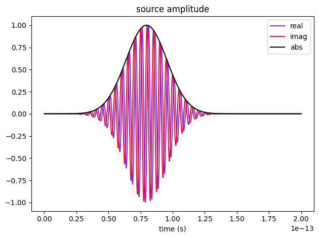
Next, we define a source injecting a normal-incidence plane-wave from above. The time dependence of the source is a Gaussian pulse. A source can be added to multiple simulations. After we add the source to a specific simulation, such that the total run time is known, we can use in-built plotting tools to visualize its time- and frequency-dependence, which we will show below.
[5]:
psource = td.PlaneWave(
    center=(0, 0, 1.5),
    direction="-",
    size=(td.inf, td.inf, 0),
    source_time=td.GaussianPulse(freq0=freq0, fwidth=fwidth),
    pol_angle=np.pi / 2,
)
Monitors#
Finally, we can also add some monitors that will record the fields that we request during the simulation run.
The two monitor types for measuring fields are FieldMonitor and FieldTimeMonitor, which record the frequency-domain and time-domain fields, respectively.
FieldMonitor objects operate by running a discrete Fourier transform of the fields at a given set of frequencies to perform the calculation “in-place” with the time stepping. FieldMonitor objects are useful for investigating the steady-state field distribution in 2D or even 3D regions of the simulation.
FieldMonitor objects are best used to monitor the time dependence of the fields at a single point, but they can also be used to create “animations” of the field pattern evolution. Because spatially large FieldMonitor objects can lead to a very large amount of data that needs to be stored, an
optional start and stop time can be supplied, as well as an interval specifying the amount of time steps between each measurement (default of 1).
[6]:
# measure time domain fields at center location, measure every 5 time steps
time_mnt = td.FieldTimeMonitor(
    center=[0, 0, 0], size=[0, 0, 0], interval=5, name="field_time"
)

# measure the steady state fields at central frequency in the xy plane and the xz plane.
freq_mnt1 = td.FieldMonitor(
    center=[0, 0, -1], size=[20, 20, 0], freqs=[freq0], name="field1"
)
freq_mnt2 = td.FieldMonitor(
    center=[0, 0, 0], size=[20, 0, 20], freqs=[freq0], name="field2"
)
Simulation#
Now we can initialize the Simulation with all the elements defined above. A nonuniform simulation grid is generated automatically based on a given minimum number of cells per wavelength in each material (10 by default), using the frequencies defined in the source.
[7]:
# Initialize simulation
sim = td.Simulation(
    size=sim_size,
    grid_spec=td.GridSpec.auto(min_steps_per_wvl=20),
    structures=[box, poly],
    sources=[psource],
    monitors=[time_mnt, freq_mnt1, freq_mnt2],
    run_time=run_time,
    boundary_spec=boundary_spec,
)
We can check the simulation monitors just to make sure everything looks right.
[8]:
for m in sim.monitors:
    m.help()
╭───────────── <class 'tidy3d.components.monitor.FieldTimeMonitor'> ─────────────╮
│ :class:`Monitor` that records electromagnetic fields in the time domain.       │
│                                                                                │
│ ╭────────────────────────────────────────────────────────────────────────────╮ │
│ │ FieldTimeMonitor(                                                          │ │
│ │ │   type='FieldTimeMonitor',                                               │ │
│ │ │   center=(0.0, 0.0, 0.0),                                                │ │
│ │ │   size=(0.0, 0.0, 0.0),                                                  │ │
│ │ │   name='field_time',                                                     │ │
│ │ │   start=0.0,                                                             │ │
│ │ │   stop=None,                                                             │ │
│ │ │   interval=5,                                                            │ │
│ │ │   fields=('Ex', 'Ey', 'Ez', 'Hx', 'Hy', 'Hz'),                           │ │
│ │ │   interval_space=(1, 1, 1),                                              │ │
│ │ │   colocate=False                                                         │ │
│ │ )                                                                          │ │
│ ╰────────────────────────────────────────────────────────────────────────────╯ │
│                                                                                │
│   bounding_box = Box(type='Box', center=(0.0, 0.0, 0.0), size=(0.0, 0.0, 0.0)) │
│         bounds = ((0.0, 0.0, 0.0), (0.0, 0.0, 0.0))                            │
│         center = (0.0, 0.0, 0.0)                                               │
│       colocate = False                                                         │
│         fields = ('Ex', 'Ey', 'Ez', 'Hx', 'Hy', 'Hz')                          │
│       geometry = Box(type='Box', center=(0.0, 0.0, 0.0), size=(0.0, 0.0, 0.0)) │
│       interval = 5                                                             │
│ interval_space = (1, 1, 1)                                                     │
│           name = 'field_time'                                                  │
│    plot_params = PlotParams(                                                   │
│                      alpha=0.4,                                                │
│                      edgecolor='orange',                                       │
│                      facecolor='orange',                                       │
│                      fill=True,                                                │
│                      hatch=None,                                               │
│                      linewidth=3.0,                                            │
│                      type='PlotParams'                                         │
│                  )                                                             │
│           size = (0.0, 0.0, 0.0)                                               │
│          start = 0.0                                                           │
│           stop = None                                                          │
│           type = 'FieldTimeMonitor'                                            │
│      zero_dims = [0, 1, 2]                                                     │
╰────────────────────────────────────────────────────────────────────────────────╯
╭─────────────────────── <class 'tidy3d.components.monitor.FieldMonitor'> ───────────────────────╮
│ :class:`Monitor` that records electromagnetic fields in the frequency domain.                  │
│                                                                                                │
│ ╭────────────────────────────────────────────────────────────────────────────────────────────╮ │
│ │ FieldMonitor(                                                                              │ │
│ │ │   type='FieldMonitor',                                                                   │ │
│ │ │   center=(0.0, 0.0, -1.0),                                                               │ │
│ │ │   size=(20.0, 20.0, 0.0),                                                                │ │
│ │ │   name='field1',                                                                         │ │
│ │ │   freqs=(200000000000000.0,),                                                            │ │
│ │ │   apodization=ApodizationSpec(                                                           │ │
│ │ │   │   start=None,                                                                        │ │
│ │ │   │   end=None,                                                                          │ │
│ │ │   │   width=None,                                                                        │ │
│ │ │   │   type='ApodizationSpec'                                                             │ │
│ │ │   ),                                                                                     │ │
│ │ │   fields=('Ex', 'Ey', 'Ez', 'Hx', 'Hy', 'Hz'),                                           │ │
│ │ │   interval_space=(1, 1, 1),                                                              │ │
│ │ │   colocate=False                                                                         │ │
│ │ )                                                                                          │ │
│ ╰────────────────────────────────────────────────────────────────────────────────────────────╯ │
│                                                                                                │
│    apodization = ApodizationSpec(start=None, end=None, width=None, type='ApodizationSpec')     │
│   bounding_box = Box(type='Box', center=(0.0, 0.0, -1.0), size=(20.0, 20.0, 0.0))              │
│         bounds = ((-10.0, -10.0, -1.0), (10.0, 10.0, -1.0))                                    │
│         center = (0.0, 0.0, -1.0)                                                              │
│       colocate = False                                                                         │
│         fields = ('Ex', 'Ey', 'Ez', 'Hx', 'Hy', 'Hz')                                          │
│          freqs = (200000000000000.0,)                                                          │
│       geometry = Box(type='Box', center=(0.0, 0.0, -1.0), size=(20.0, 20.0, 0.0))              │
│ interval_space = (1, 1, 1)                                                                     │
│           name = 'field1'                                                                      │
│    plot_params = PlotParams(                                                                   │
│                      alpha=0.4,                                                                │
│                      edgecolor='orange',                                                       │
│                      facecolor='orange',                                                       │
│                      fill=True,                                                                │
│                      hatch=None,                                                               │
│                      linewidth=3.0,                                                            │
│                      type='PlotParams'                                                         │
│                  )                                                                             │
│           size = (20.0, 20.0, 0.0)                                                             │
│           type = 'FieldMonitor'                                                                │
│      zero_dims = [2]                                                                           │
╰────────────────────────────────────────────────────────────────────────────────────────────────╯
╭─────────────────────── <class 'tidy3d.components.monitor.FieldMonitor'> ───────────────────────╮
│ :class:`Monitor` that records electromagnetic fields in the frequency domain.                  │
│                                                                                                │
│ ╭────────────────────────────────────────────────────────────────────────────────────────────╮ │
│ │ FieldMonitor(                                                                              │ │
│ │ │   type='FieldMonitor',                                                                   │ │
│ │ │   center=(0.0, 0.0, 0.0),                                                                │ │
│ │ │   size=(20.0, 0.0, 20.0),                                                                │ │
│ │ │   name='field2',                                                                         │ │
│ │ │   freqs=(200000000000000.0,),                                                            │ │
│ │ │   apodization=ApodizationSpec(                                                           │ │
│ │ │   │   start=None,                                                                        │ │
│ │ │   │   end=None,                                                                          │ │
│ │ │   │   width=None,                                                                        │ │
│ │ │   │   type='ApodizationSpec'                                                             │ │
│ │ │   ),                                                                                     │ │
│ │ │   fields=('Ex', 'Ey', 'Ez', 'Hx', 'Hy', 'Hz'),                                           │ │
│ │ │   interval_space=(1, 1, 1),                                                              │ │
│ │ │   colocate=False                                                                         │ │
│ │ )                                                                                          │ │
│ ╰────────────────────────────────────────────────────────────────────────────────────────────╯ │
│                                                                                                │
│    apodization = ApodizationSpec(start=None, end=None, width=None, type='ApodizationSpec')     │
│   bounding_box = Box(type='Box', center=(0.0, 0.0, 0.0), size=(20.0, 0.0, 20.0))               │
│         bounds = ((-10.0, 0.0, -10.0), (10.0, 0.0, 10.0))                                      │
│         center = (0.0, 0.0, 0.0)                                                               │
│       colocate = False                                                                         │
│         fields = ('Ex', 'Ey', 'Ez', 'Hx', 'Hy', 'Hz')                                          │
│          freqs = (200000000000000.0,)                                                          │
│       geometry = Box(type='Box', center=(0.0, 0.0, 0.0), size=(20.0, 0.0, 20.0))               │
│ interval_space = (1, 1, 1)                                                                     │
│           name = 'field2'                                                                      │
│    plot_params = PlotParams(                                                                   │
│                      alpha=0.4,                                                                │
│                      edgecolor='orange',                                                       │
│                      facecolor='orange',                                                       │
│                      fill=True,                                                                │
│                      hatch=None,                                                               │
│                      linewidth=3.0,                                                            │
│                      type='PlotParams'                                                         │
│                  )                                                                             │
│           size = (20.0, 0.0, 20.0)                                                             │
│           type = 'FieldMonitor'                                                                │
│      zero_dims = [1]                                                                           │
╰────────────────────────────────────────────────────────────────────────────────────────────────╯
Visualization functions#
We can now use the some in-built plotting functions to make sure that we have set up the simulation as we desire.
First, let’s take a look at the source time dependence.
[9]:
# Visualize source
psource.source_time.plot(np.linspace(0, run_time, 1001))
plt.show()
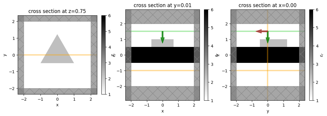
And now let’s visualize the simulation.
For this, we will plot three cross sections at z=0.75, y=0, and x=0, respectively.
The relative permittivity of objects is plotted in greyscale.
By default, sources are overlayed in green, monitors in yellow, and PML boundaries in grey.
[10]:
fig, ax = plt.subplots(1, 3, figsize=(13, 4))
sim.plot_eps(z=0.75, freq=freq0, ax=ax[0])
sim.plot_eps(y=0.01, freq=freq0, ax=ax[1])
sim.plot_eps(x=0, freq=freq0, ax=ax[2])
[00:00:27] INFO Auto meshing using wavelength 1.4990 defined from sources. grid_spec.py:510
[10]:
<AxesSubplot: title={'center': 'cross section at x=0.00'}, xlabel='y', ylabel='z'>
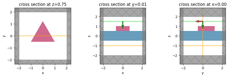
Alternatively, we can also plot the structures with a fake color based on the material they are made of.
[11]:
fig, ax = plt.subplots(1, 3, figsize=(12, 3))
sim.plot(z=0.75, ax=ax[0])
sim.plot(y=0.01, ax=ax[1])
sim.plot(x=0, ax=ax[2])
[11]:
<AxesSubplot: title={'center': 'cross section at x=0.00'}, xlabel='y', ylabel='z'>
Running through the web API#
Now that the simulation is constructed, we can run it using the web API of Tidy3D. First, we submit the project. Note that we can give it a custom name.
[12]:
task_id = web.upload(sim, task_name="Simulation")
The task is still in draft status and will not run until we call the start function. Before that, we may want to check the estimated cost of the task.
[13]:
print("Max flex unit cost: ", web.estimate_cost(task_id))
Max flex unit cost: 0.025
We can now start the task, and if we want to, continously monitor its status, and wait until the run is successful. The monitor function will keep running until either a 'success' or 'error' status is returned.
[14]:
web.start(task_id)
web.monitor(task_id)
Loading and analyzing data#
After a successful run, we can download the results and load them into our simulation model. We use the download_results function from our web API, which downloads a single hdf5 file containing all the monitor data, a log file, and a json file defining the original simulation (same as what you’ll get if you run sim.to_json() on the current object). Optionally, you can provide a folder in which to store the files. In the example below, the results are stored in the data/
folder.
[15]:
sim_data = web.load(task_id, path="data/sim_data.hdf5")

# Show the output of the log file
print(sim_data.log)
Simulation domain Nx, Ny, Nz: [156, 157, 104]
Applied symmetries: (0, 0, 0)
Number of computational grid points: 2.6629e+06.
Using subpixel averaging: True
Number of time steps: 3.4930e+03
Automatic shutoff factor: 1.00e-05
Time step (s): 5.7275e-17


Compute source modes time (s):     0.1773
Compute monitor modes time (s):    0.0023
Rest of setup time (s):            2.2910

Running solver for 3493 time steps...
- Time step    139 / time 7.96e-15s (  4 % done), field decay: 1.00e+00
- Time step    279 / time 1.60e-14s (  8 % done), field decay: 1.00e+00
- Time step    419 / time 2.40e-14s ( 12 % done), field decay: 1.00e+00
- Time step    558 / time 3.20e-14s ( 16 % done), field decay: 1.00e+00
- Time step    698 / time 4.00e-14s ( 20 % done), field decay: 1.00e+00
- Time step    838 / time 4.80e-14s ( 24 % done), field decay: 1.00e+00
- Time step    978 / time 5.60e-14s ( 28 % done), field decay: 1.00e+00
- Time step   1117 / time 6.40e-14s ( 32 % done), field decay: 1.00e+00
- Time step   1257 / time 7.20e-14s ( 36 % done), field decay: 1.00e+00
- Time step   1389 / time 7.96e-14s ( 39 % done), field decay: 1.00e+00
- Time step   1397 / time 8.00e-14s ( 40 % done), field decay: 1.00e+00
- Time step   1536 / time 8.80e-14s ( 44 % done), field decay: 1.00e+00
- Time step   1676 / time 9.60e-14s ( 48 % done), field decay: 8.05e-01
- Time step   1816 / time 1.04e-13s ( 52 % done), field decay: 3.46e-01
- Time step   1956 / time 1.12e-13s ( 56 % done), field decay: 1.51e-01
- Time step   2095 / time 1.20e-13s ( 60 % done), field decay: 5.29e-02
- Time step   2235 / time 1.28e-13s ( 64 % done), field decay: 1.21e-02
- Time step   2375 / time 1.36e-13s ( 68 % done), field decay: 2.31e-03
- Time step   2514 / time 1.44e-13s ( 72 % done), field decay: 4.89e-04
- Time step   2654 / time 1.52e-13s ( 76 % done), field decay: 1.11e-04
- Time step   2794 / time 1.60e-13s ( 80 % done), field decay: 2.39e-05
- Time step   2934 / time 1.68e-13s ( 84 % done), field decay: 4.75e-06
Field decay smaller than shutoff factor, exiting solver.

Solver time (s):                   5.0762
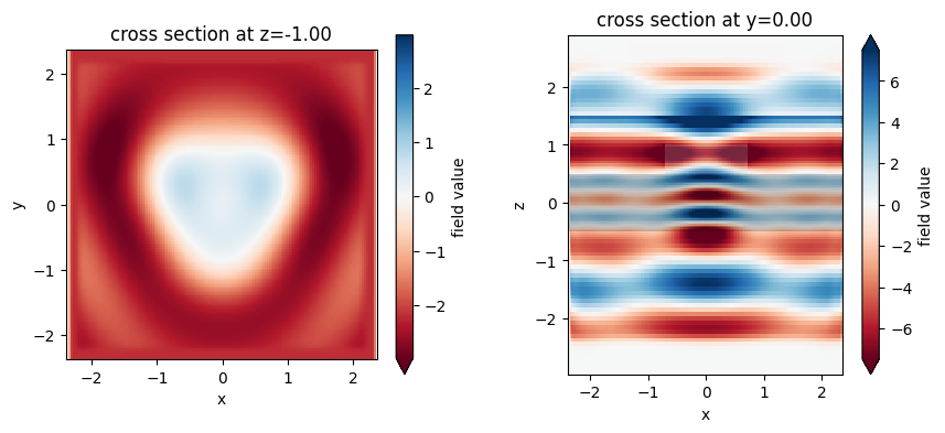
Visualization functions#
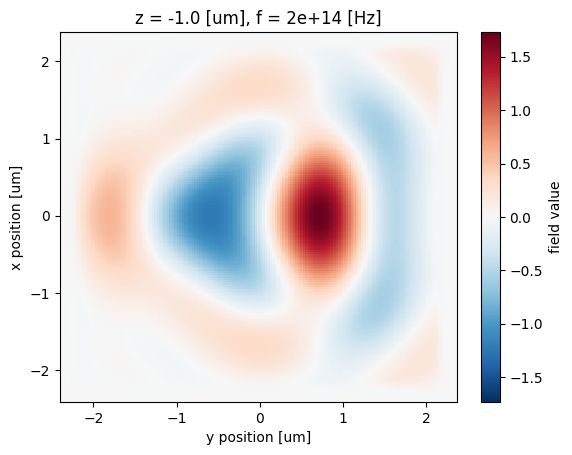
Finally, we can now use the in-built visualization tools to examine the results. Below, we plot the y-component of the field recorded by the two frequency monitors (this is the dominant component since the source is y-polarized).
[16]:
fig, ax = plt.subplots(1, 2, figsize=(10, 4))
sim_data.plot_field("field1", "Ey", z=-1.0, ax=ax[0], val="real")
sim_data.plot_field("field2", "Ey", ax=ax[1], val="real")
INFO Auto meshing using wavelength 1.4990 defined from sources. grid_spec.py:510
[16]:
<AxesSubplot: title={'center': 'cross section at y=0.00'}, xlabel='x', ylabel='z'>
Monitor data#
The raw field data can be accessed through indexing by monitor name directly.
For plenty of discussion on accessing and manipulating data, refer to the data visualization tutorial.
[17]:
mon1_data = sim_data["field1"]
mon1_data.Ex
[17]:
<xarray.ScalarFieldDataArray (x: 158, y: 159, z: 1, f: 1)>
array([[[[ 0.0000000e+00+0.0000000e+00j]],

        [[ 0.0000000e+00+0.0000000e+00j]],

        [[ 9.8186092e-07+4.0431851e-07j]],

        ...,

        [[ 9.9795454e-07+1.7111465e-07j]],

        [[ 1.2159646e-07+6.0561064e-08j]],

        [[ 0.0000000e+00+0.0000000e+00j]]],


       [[[ 0.0000000e+00+0.0000000e+00j]],

        [[ 0.0000000e+00+0.0000000e+00j]],

        [[ 9.8186092e-07+4.0431851e-07j]],
...
        [[-1.1717159e-07+2.6605029e-08j]],

        [[ 8.6237844e-09-7.4280364e-09j]],

        [[ 0.0000000e+00+0.0000000e+00j]]],


       [[[ 0.0000000e+00+0.0000000e+00j]],

        [[ 0.0000000e+00+0.0000000e+00j]],

        [[-8.3378872e-08+3.6394130e-08j]],

        ...,

        [[-1.1717159e-07+2.6605029e-08j]],

        [[ 8.6237844e-09-7.4280364e-09j]],

        [[ 0.0000000e+00+0.0000000e+00j]]]], dtype=complex64)
Coordinates:
  * x        (x) float64 -2.379 -2.348 -2.318 -2.288 ... 2.288 2.318 2.348 2.379
  * y        (y) float64 -2.39 -2.36 -2.33 -2.3 ... 2.266 2.295 2.325 2.354
  * z        (z) float64 -1.0
  * f        (f) float64 2e+14
Attributes:
long_name: field value[18]:
ax = mon1_data.Ez.real.plot()
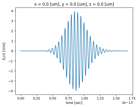
We can use this raw data for example to also plot the time-domain fields recorded in the FieldTimeMonitor, which look largely like a delayed version of the source input, indicating that no resonant features were excited.
[19]:
time_data = sim_data["field_time"]
fig, ax = plt.subplots(1)
time_data.Ey.plot()
ax.set_ylabel("$E_y(t)$ [V/m]")
plt.show()
Permittivity data#
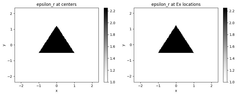
We can also query the relative permittivity in the simulation within a volume parameterized by a td.Box. The method Simulation.epsilon(box, coord_key) returns the permittivity within the specified volume.
The coord_key specifies at what locations in the yee cell to evaluate the permittivity at (eg. 'centers', 'Ey', 'Hz', etc.).
[20]:
volume = td.Box(center=(0, 0, 0.75), size=(5, 5, 0))

# at Yee cell centers
eps_centers = sim.epsilon(box=volume, coord_key="centers")

# at Ex locations in the yee cell
eps_Ex = sim.epsilon(box=volume, coord_key="Ex")
Return an xarray DataArray containing the complex-valued permittivity values at the Yee cell centers and the “Ex” within the box.
We can then plot or post-process this data as we wish.
[21]:
f, (ax1, ax2) = plt.subplots(1, 2, tight_layout=True, figsize=(10, 4))

eps_centers.real.plot(x="x", y="y", cmap="Greys", ax=ax1)
eps_Ex.real.plot(x="x", y="y", cmap="Greys", ax=ax2)
ax1.set_title("epsilon_r at centers")
ax2.set_title("epsilon_r at Ex locations")

plt.show()
[ ]: