Plastic biosensor grating
Contents
Plastic biosensor grating#
Note: the cost of running the entire notebook is larger than 1 FlexUnit.
Bragg gratings are structures which involve a periodic variation in the refractive index or geometry of waveguide, so that certain frequencies of light are reflected off the grating while others are transmitted.
Since gratings can be designed to be extremely sentitive to a narrow band of frequencies, one possible application is to detect the presence of foreign molecules. If particles such as biomolecules are deposited on the device, it will no longer have the same reflective properties in the narrow band of frequencies for which it was designed. Therefore, carefully-designed Bragg gratings can be used as biosensors.
In this example, an optical biosensor grating is modeled to detect the presence of biomolecules. The grating is designed to be reflective over a narrow band around its resonant frequency which is modified by the presence of a biomolecule.
Reference: Brian Cunningham, Bo Lin, Jean Qiu, Peter Li, Jane Pepper, Brenda Hugh, “A plastic colorimetric resonant optical biosensor for multiparallel detection of label-free biochemical interactions,” Sensors and Actuators B 85 (2002)
[1]:
# basic imports
import numpy as np
import matplotlib.pylab as plt

# tidy3d imports
import tidy3d as td
[19:47:03] WARNING  This version of Tidy3D was pip installed from the 'tidy3d-beta' repository on   __init__.py:103
                    PyPI. Future releases will be uploaded to the 'tidy3d' repository. From now on,
                    please use 'pip install tidy3d' instead.
INFO Using client version: 1.9.0rc1 __init__.py:121
Structure Setup#
Create the grating geometry.
[2]:
# materials
Si3N4 = td.Medium(permittivity=2.05**2)
epoxy = td.Medium(permittivity=1.5**2)
water = td.Medium(permittivity=1.333**2)
# substrate = td.material_library['Polycarbonate']['Sultanova2009']
substrate = td.Medium(permittivity=1.333**2)

# set basic geometric parameters (units in microns)
nm = 1e-3
period = 550 * nm
grating_ratio = 0.5
num_periods = 10
grating_height = 200 * nm
film_height = 120 * nm
epoxy_height = 400 * nm
buffer = 0.1
substrate_height = 1.5
substrate_width = 7.0
sim_size = (num_periods * period, substrate_width, 2 * substrate_height)
# sim_size = (num_periods * period + 450 * nm, substrate_width, 2 * substrate_height)
grating_size = (period * grating_ratio, td.inf, grating_height)
film_high_size = (period * grating_ratio, td.inf, film_height)
film_low_size = (period * (1.0 - grating_ratio), td.inf, film_height)

# wavelength / frequency setup
wavelength_min = 780 * nm
wavelength_max = 900 * nm
freq_min = td.C_0 / wavelength_max
freq_max = td.C_0 / wavelength_min
freq0 = (freq_min + freq_max) / 2.0
fwidth = freq_max - freq_min
run_time = 4e-12

# create the substrate
substrate = td.Structure(
    geometry=td.Box(
        center=[0.0, 0.0, -substrate_height / 2.0 - buffer / 2.0],
        # size=[num_periods * period + buffer, td.inf, substrate_height + buffer],
        size=[td.inf, td.inf, substrate_height + buffer],
    ),
    medium=substrate,
    name="substrate",
)

# create the epoxy layer
epoxy_layer = td.Structure(
    geometry=td.Box(
        center=[0.0, 0.0, epoxy_height / 2.0],
        # size=[num_periods * period + buffer, td.inf, epoxy_height],
        size=[td.inf, td.inf, epoxy_height],
    ),
    medium=epoxy,
    name="epoxy_layer",
)

# create the grating with the Si3N4 film
gratings = []
films_high = []
films_low = []
for i in range(num_periods):
    grating_center = [
        -sim_size[0] / 2.0 + period * grating_ratio / 2.0 + i * period,
        0.0,
        epoxy_height + grating_height / 2.0,
    ]
    size = list(grating_size)
    if i == 0:
        grating_center[0] -= buffer / 2.0
        size[0] += buffer
    grating = td.Structure(
        geometry=td.Box(center=grating_center, size=size),
        medium=epoxy,
        name=f"grating_{i}",
    )

    film_high_center = [
        -sim_size[0] / 2.0 + period * grating_ratio / 2.0 + i * period,
        0.0,
        epoxy_height + grating_height + film_height / 2.0,
    ]
    size = list(film_high_size)
    if i == 0:
        film_high_center[0] -= buffer / 2.0
        size[0] += buffer
    film_high = td.Structure(
        geometry=td.Box(center=film_high_center, size=size),
        medium=Si3N4,
        name=f"film_high_{i}",
    )

    film_low_center = [
        -sim_size[0] / 2.0
        + period * grating_ratio
        + period * (1.0 - grating_ratio) / 2.0
        + i * period,
        0.0,
        epoxy_height + film_height / 2.0,
    ]
    size = list(film_low_size)
    if i == num_periods - 1:
        film_low_center[0] += buffer / 2.0
        size[0] += buffer
    film_low = td.Structure(
        geometry=td.Box(center=film_low_center, size=size),
        medium=Si3N4,
        name=f"film_low_{i}",
    )

    gratings.append(grating)
    films_high.append(film_high)
    films_low.append(film_low)

geometry = [substrate, epoxy_layer] + gratings + films_high + films_low

# boundary conditions
boundary_spec = td.BoundarySpec(
    x=td.Boundary.periodic(),
    # x=td.Boundary.pml(),
    y=td.Boundary.pml(),
    z=td.Boundary.pml(),
)

# grid specification
grid_spec = td.GridSpec.auto(min_steps_per_wvl=30)
Source Setup#
Create the plane wave source which excites the structure from underneath.
[3]:
source_time = td.GaussianPulse(freq0=freq0, fwidth=fwidth)
source = td.PlaneWave(
    center=[0, 0, -0.5 * substrate_height],
    size=[td.inf, td.inf, 0.0],
    source_time=source_time,
    pol_angle=0,
    direction="+",
)
Monitor Setup#
Create field and flux monitors to measure reflecting and transmitted flux.
[4]:
# create field monitor
monitor_xy = td.FieldMonitor(
    center=[0, 0, epoxy_height + film_height / 2],
    size=[td.inf, td.inf, 0],
    freqs=[freq0],
    name="fields_xy",
)

# create flux monitors
freqs = list(np.linspace(freq_min, freq_max, 1000))
monitor_flux_refl = td.FluxMonitor(
    center=[0, 0, -0.75 * substrate_height],
    size=[td.inf, td.inf, 0.0],
    freqs=freqs,
    name="flux_refl",
)
monitor_flux_tran = td.FluxMonitor(
    center=[0, 0, 0.75 * substrate_height],
    size=[td.inf, td.inf, 0.0],
    freqs=freqs,
    name="flux_tran",
)

monitors = [monitor_xy, monitor_flux_refl, monitor_flux_tran]
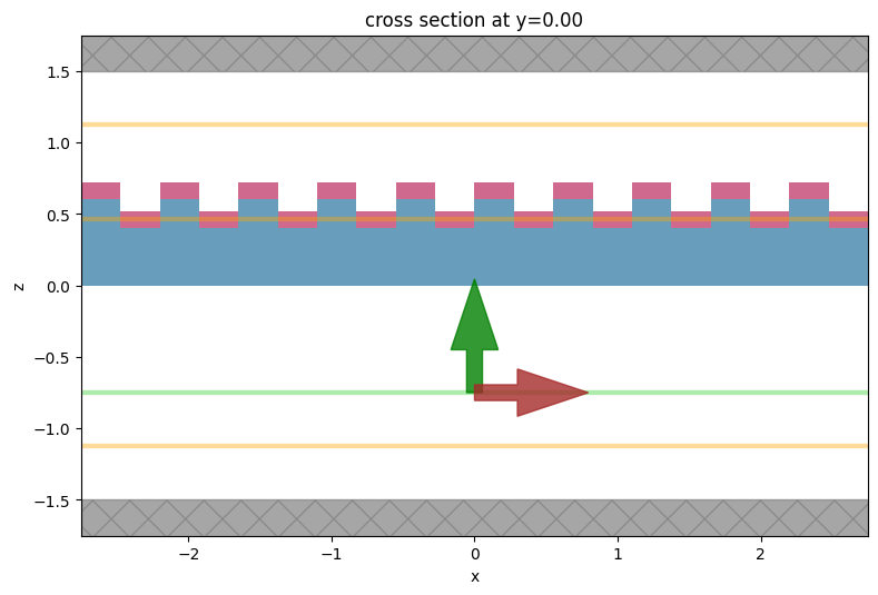
Create Simulation#
The final simulation object is created and visualized.
[5]:
# create the simulation
sim = td.Simulation(
    center=[0, 0, 0],
    size=sim_size,
    grid_spec=grid_spec,
    structures=geometry,
    sources=[source],
    monitors=monitors,
    run_time=run_time,
    boundary_spec=boundary_spec,
    medium=water,
    shutoff=1e-6,
)

# plot the simulation domain
f, ax = plt.subplots(tight_layout=True, figsize=(8, 6))
sim.plot(y=0, ax=ax)
INFO Auto meshing using wavelength 0.8357 defined from sources. grid_spec.py:510
[5]:
<AxesSubplot: title={'center': 'cross section at y=0.00'}, xlabel='x', ylabel='z'>
Run Simulation#
[6]:
# run simulation
import tidy3d.web as web

sim_data = web.run(sim, task_name="biosensor", path="data/biosensor.hdf5")
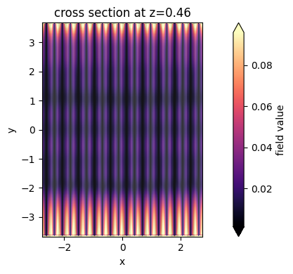
Plot Fields#
The frequency-domain fields recorded are plotted at the center frequency in an xy plane cutting through the grating.
[7]:
# plot fields on the monitor
fig, ax = plt.subplots(tight_layout=True, figsize=(9, 4))
sim_data.plot_field(
    field_monitor_name="fields_xy", field_name="Ey", val="abs", f=freq0, ax=ax
)
[19:53:58] INFO Auto meshing using wavelength 0.8357 defined from sources. grid_spec.py:510
[7]:
<AxesSubplot: title={'center': 'cross section at z=0.46'}, xlabel='x', ylabel='y'>
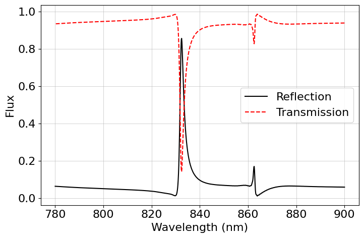
Plot Transmission and Reflection#
To see the effectiveness of the grating, we can compute and plot the reflection and transmission via the flux measured by the flux monitor. As is visible in the plot, the structure is highly reflective in a narrow frequency band around the design frequency, allowing one to detect small variations in the frequency response due to the presence of biological materials.
[8]:
plt.rcParams.update({"font.size": 16})

transmission = sim_data["flux_tran"].flux
reflection = 1 - transmission

fig, ax = plt.subplots(figsize=(7.5, 5))
ax.plot(td.C_0 / freqs * 1e3, reflection, "-k", label="Reflection")
ax.plot(td.C_0 / freqs * 1e3, transmission, "--r", label="Transmission")
ax.set(
    xlabel="Wavelength (nm)",
    ylabel="Flux",
    yscale="linear",
    xscale="linear",
    # xlim = [500, 550]
)
ax.legend()
ax.grid(visible=True, which="both", axis="both", linewidth=0.4)
plt.tight_layout()
[ ]: