Grating coupler
Contents
Grating coupler#
[1]:
# basic imports
import numpy as np
import matplotlib.pylab as plt

# tidy3d imports
import tidy3d as td
import tidy3d.web as web
[21:37:16] WARNING  This version of Tidy3D was pip installed from the 'tidy3d-beta' repository on   __init__.py:103
                    PyPI. Future releases will be uploaded to the 'tidy3d' repository. From now on,
                    please use 'pip install tidy3d' instead.
INFO Using client version: 1.9.0rc1 __init__.py:121
Problem Setup#
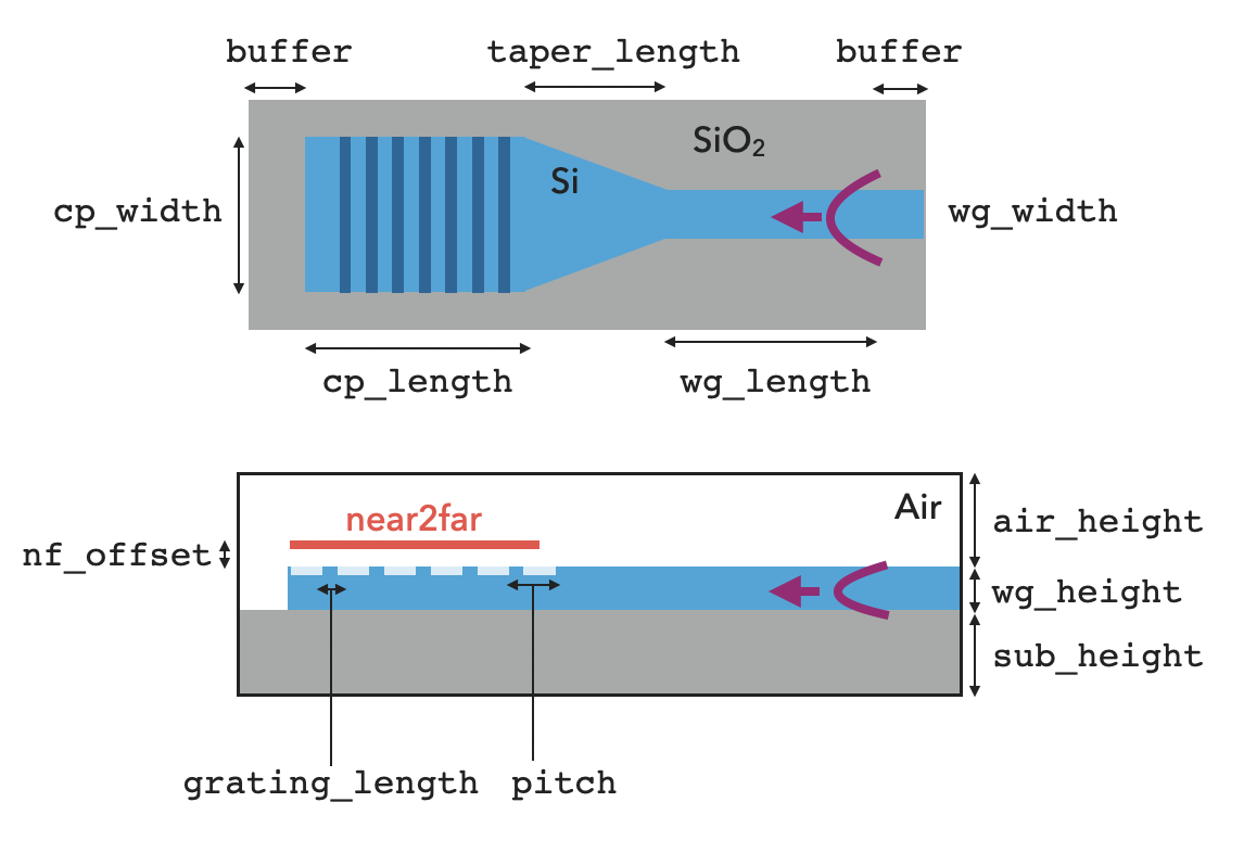
In this example, we model a 3D grating coupler in a Silicon on Insulator (SOI) platform.
A basic schematic of the design is shown below. The simulation is about 19um x 4um x 5um with a wavelength of 1.55um and takes about 1 minute to simulate 10,000 time steps.
In the simulation, we inject a modal source into the waveguide and propagate it towards the grating structure. The radiation from the grating coupler is then measured with a near field monitor and we use a far field projection to inspect the angular dependence of the radiation.
[2]:
# basic parameters (note, all length units are microns)
nm = 1e-3
wavelength = 1550 * nm

# grid specification
grid_spec = td.GridSpec.auto(min_steps_per_wvl=20, wavelength=wavelength)

# waveguide
wg_width = 400 * nm
wg_height = 220 * nm
wg_length = 2 * wavelength

# surrounding
sub_height = 2.0
air_height = 2.0
buffer = 0.5 * wavelength

# coupler
cp_width = 4 * wavelength
cp_length = 8 * wavelength
taper_length = 6 * wavelength
[3]:
# sizes
Lx = buffer + wg_length + taper_length + cp_length
Ly = buffer + cp_width + buffer
Lz = sub_height + wg_height + air_height
sim_size = [Lx, Ly, Lz]

# convenience variables to store center of coupler and waveguide
wg_center_x = +Lx / 2 - buffer - (wg_length + taper_length) / 2
cp_center_x = -Lx / 2 + buffer + cp_length / 2
wg_center_z = -Lz / 2 + sub_height + wg_height / 2
cp_center_z = -Lz / 2 + sub_height + wg_height / 2

# materials
Air = td.Medium(permittivity=1.0)
Si = td.Medium(permittivity=3.47**2)
SiO2 = td.Medium(permittivity=1.44**2)

# source parameters
freq0 = td.C_0 / wavelength
fwidth = freq0 / 10
run_time = 100 / fwidth
Mode Solve#
To determine the pitch of the waveguide for a given design angle, we need to compute the effective index of the waveguide mode being coupled into. For this, we set up a simple simulation of the coupler region and use the mode solver to get the effective index. We will not run this simulation, we just add a ModeMonitor object in order to call the mode solver, sim.compute_modes() below, and get the effective index of the wide-waveguide region.
[4]:
# grating parameters
design_theta_deg = -30
design_theta_rad = np.pi * design_theta_deg / 180
grating_height = 70 * nm
# do a mode solve to get neff of the coupler
sub = td.Structure(
geometry=td.Box(center=[0, 0, -Lz / 2], size=[td.inf, td.inf, 2 * sub_height]),
medium=SiO2,
name="substrate",
)
cp = td.Structure(
geometry=td.Box(
center=[0, 0, cp_center_z - grating_height / 4],
size=[td.inf, cp_width, wg_height - grating_height / 2],
),
medium=Si,
name="coupler",
)
mode_plane = td.Box(center=(0, 0, 0), size=(0, 8 * cp_width, 8 * wg_height))
sim = td.Simulation(
size=sim_size,
grid_spec=grid_spec,
structures=[sub, cp],
sources=[],
monitors=[],
boundary_spec=td.BoundarySpec.all_sides(boundary=td.PML()),
run_time=1e-12,
)
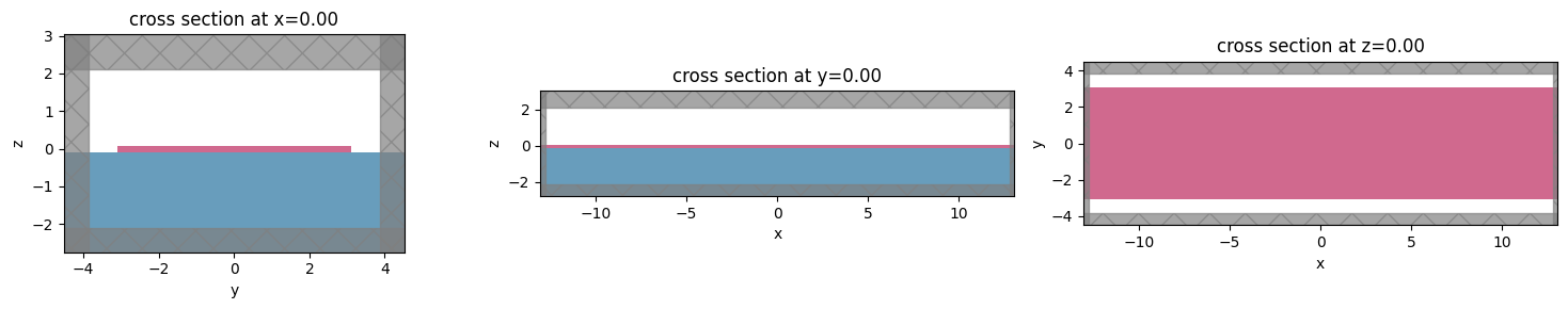
f, (ax1, ax2, ax3) = plt.subplots(1, 3, tight_layout=True, figsize=(15, 3))
sim.plot(x=0, ax=ax1)
sim.plot(y=0, ax=ax2)
sim.plot(z=0, ax=ax3)
[21:37:17] WARNING No sources in simulation. simulation.py:494
[4]:
<AxesSubplot: title={'center': 'cross section at z=0.00'}, xlabel='x', ylabel='y'>
Compute Effective index for Grating Pitch Design#
[5]:
from tidy3d.plugins import ModeSolver

ms = ModeSolver(
    simulation=sim, plane=mode_plane, mode_spec=td.ModeSpec(), freqs=[freq0]
)
mode_output = ms.solve()
/Users/twhughes/.pyenv/versions/3.10.9/lib/python3.10/site-packages/numpy/linalg/linalg.py:2139: RuntimeWarning: divide by zero encountered in det
  r = _umath_linalg.det(a, signature=signature)
/Users/twhughes/.pyenv/versions/3.10.9/lib/python3.10/site-packages/numpy/linalg/linalg.py:2139: RuntimeWarning: invalid value encountered in det
  r = _umath_linalg.det(a, signature=signature)
[6]:
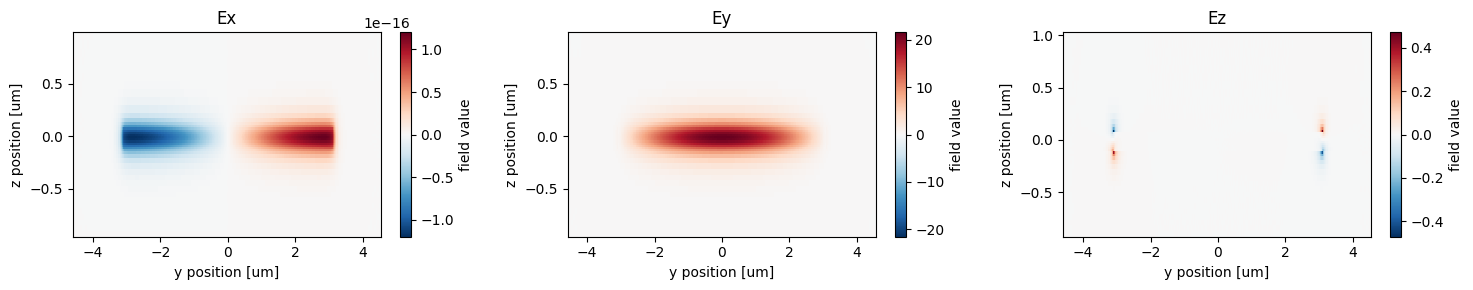
f, (ax1, ax2, ax3) = plt.subplots(1, 3, tight_layout=True, figsize=(15, 3))
mode_output.Ex.real.plot(x="y", y="z", ax=ax1)
mode_output.Ey.real.plot(x="y", y="z", ax=ax2)
mode_output.Ez.real.plot(x="y", y="z", ax=ax3)
ax1.set_title("Ex")
ax2.set_title("Ey")
ax3.set_title("Ez")
plt.show()
[7]:
neff = float(mode_output.n_eff)
print(f"effective index = {neff:.4f}")
effective index = 2.6885
Create Simulation#
Now we set up the grating coupler to simulate in Tidy3D.
[8]:
# gratings
pitch = wavelength / (neff - np.sin(abs(design_theta_rad)))
grating_length = pitch / 2.0
num_gratings = int(cp_length / pitch)

sub = td.Structure(
    geometry=td.Box(
        center=[0, 0, -Lz / 2],
        size=[td.inf, td.inf, 2 * sub_height],
    ),
    medium=SiO2,
    name="substrate",
)

wg = td.Structure(
    geometry=td.Box(
        center=[wg_center_x, 0, wg_center_z],
        size=[buffer + wg_length + taper_length + cp_length / 2, wg_width, wg_height],
    ),
    medium=Si,
    name="waveguide",
)

cp = td.Structure(
    geometry=td.Box(
        center=[cp_center_x, 0, cp_center_z],
        size=[cp_length, cp_width, wg_height],
    ),
    medium=Si,
    name="coupler",
)

tp = td.Structure(
    geometry=td.PolySlab(
        vertices=[
            [cp_center_x + cp_length / 2 + taper_length, +wg_width / 2],
            [cp_center_x + cp_length / 2 + taper_length, -wg_width / 2],
            [cp_center_x + cp_length / 2, -cp_width / 2],
            [cp_center_x + cp_length / 2, +cp_width / 2],
        ],
        slab_bounds=(wg_center_z - wg_height / 2, wg_center_z + wg_height / 2),
        axis=2,
    ),
    medium=Si,
    name="taper",
)

grating_left_x = cp_center_x - cp_length / 2
gratings = [
    td.Structure(
        geometry=td.Box(
            center=[
                grating_left_x + (i + 0.5) * pitch,
                0,
                cp_center_z + wg_height / 2 - grating_height / 2,
            ],
            size=[grating_length, cp_width, grating_height],
        ),
        medium=Air,
        name=f"{i}th_grating",
    )
    for i in range(num_gratings)
]
[9]:
# distance to near field monitor
nf_offset = 50 * nm

plane_monitor = td.FieldMonitor(
    center=[0, 0, cp_center_z],
    size=[td.inf, td.inf, 0],
    freqs=[freq0],
    name="full_domain_fields",
)

rad_monitor = td.FieldMonitor(
    center=[0, 0, 0], size=[td.inf, 0, td.inf], freqs=[freq0], name="radiated_fields"
)

near_field_monitor = td.FieldMonitor(
    center=[cp_center_x, 0, cp_center_z + wg_height / 2 + nf_offset],
    size=[td.inf, td.inf, 0],
    freqs=[freq0],
    name="radiated_near_fields",
)
[10]:
sim = td.Simulation(
    size=sim_size,
    grid_spec=grid_spec,
    structures=[sub, wg, cp, tp] + gratings,
    sources=[],
    monitors=[plane_monitor, rad_monitor, near_field_monitor],
    run_time=run_time,
    boundary_spec=td.BoundarySpec.all_sides(boundary=td.PML()),
)
[21:38:13] WARNING No sources in simulation. simulation.py:494
Make Modal Source#
[11]:
source_plane = td.Box(
center=[Lx / 2 - buffer, 0, cp_center_z],
size=[0, 8 * wg_width, 8 * wg_height],
)
ms = ModeSolver(
simulation=sim, plane=source_plane, mode_spec=td.ModeSpec(), freqs=[freq0]
)
mode_output = ms.solve()
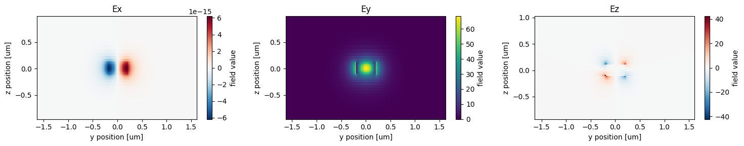
f, (ax1, ax2, ax3) = plt.subplots(1, 3, tight_layout=True, figsize=(15, 3))
mode_output.Ex.real.plot(x="y", y="z", ax=ax1)
mode_output.Ey.real.plot(x="y", y="z", ax=ax2)
mode_output.Ez.real.plot(x="y", y="z", ax=ax3)
ax1.set_title("Ex")
ax2.set_title("Ey")
ax3.set_title("Ez")
plt.show()
/Users/twhughes/.pyenv/versions/3.10.9/lib/python3.10/site-packages/numpy/linalg/linalg.py:2139: RuntimeWarning: divide by zero encountered in det
  r = _umath_linalg.det(a, signature=signature)
/Users/twhughes/.pyenv/versions/3.10.9/lib/python3.10/site-packages/numpy/linalg/linalg.py:2139: RuntimeWarning: invalid value encountered in det
  r = _umath_linalg.det(a, signature=signature)
[12]:
source_time = td.GaussianPulse(freq0=freq0, fwidth=fwidth)
mode_src = ms.to_source(mode_index=0, direction="-", source_time=source_time)
sim = sim.copy(update={"sources": [mode_src]})
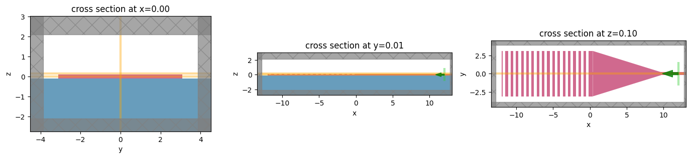
[13]:
fig, (ax1, ax2, ax3) = plt.subplots(1, 3, tight_layout=True, figsize=(14, 3))
sim.plot(x=0, ax=ax1)
sim.plot(y=0.01, ax=ax2)
sim.plot(z=0.1, ax=ax3)
plt.show()
[14]:
mode_src.help()
╭───────────────────────────────── <class 'tidy3d.components.source.ModeSource'> ─────────────────────────────────╮ │ Injects current source to excite modal profile on finite extent plane. │ │ │ │ ╭─────────────────────────────────────────────────────────────────────────────────────────────────────────────╮ │ │ │ ModeSource( │ │ │ │ │ type='ModeSource', │ │ │ │ │ center=(12.012500000000001, 0.0, -3.191891195797325e-16), │ │ │ │ │ size=(0.0, 3.2, 1.76), │ │ │ │ │ source_time=GaussianPulse( │ │ │ │ │ │ amplitude=1.0, │ │ │ │ │ │ phase=0.0, │ │ │ │ │ │ type='GaussianPulse', │ │ │ │ │ │ freq0=193414489116771.6, │ │ │ │ │ │ fwidth=19341448911677.16, │ │ │ │ │ │ offset=5.0 │ │ │ │ │ ), │ │ │ │ │ name=None, │ │ │ │ │ num_freqs=1, │ │ │ │ │ direction='-', │ │ │ │ │ mode_spec=ModeSpec( │ │ │ │ │ │ num_modes=1, │ │ │ │ │ │ target_neff=None, │ │ │ │ │ │ num_pml=(0, 0), │ │ │ │ │ │ filter_pol=None, │ │ │ │ │ │ angle_theta=0.0, │ │ │ │ │ │ angle_phi=0.0, │ │ │ │ │ │ precision='single', │ │ │ │ │ │ bend_radius=None, │ │ │ │ │ │ bend_axis=None, │ │ │ │ │ │ track_freq='central', │ │ │ │ │ │ type='ModeSpec' │ │ │ │ │ ), │ │ │ │ │ mode_index=0 │ │ │ │ ) │ │ │ ╰─────────────────────────────────────────────────────────────────────────────────────────────────────────────╯ │ │ │ │ angle_phi = 0.0 │ │ angle_theta = 0.0 │ │ bounding_box = Box( │ │ type='Box', │ │ center=( │ │ 12.012500000000001, │ │ 0.0, │ │ -3.3306690738754696e-16 │ │ ), │ │ size=(0.0, 3.2, 1.76) │ │ ) │ │ bounds = ( │ │ (12.012500000000001, -1.6, -0.8800000000000003), │ │ (12.012500000000001, 1.6, 0.8799999999999997) │ │ ) │ │ center = (12.012500000000001, 0.0, -3.191891195797325e-16) │ │ direction = '-' │ │ frequency_grid = array([1.93414489e+14]) │ │ geometry = Box( │ │ type='Box', │ │ center=(12.012500000000001, 0.0, -3.191891195797325e-16), │ │ size=(0.0, 3.2, 1.76) │ │ ) │ │ injection_axis = 0 │ │ mode_index = 0 │ │ mode_spec = ModeSpec( │ │ num_modes=1, │ │ target_neff=None, │ │ num_pml=(0, 0), │ │ filter_pol=None, │ │ angle_theta=0.0, │ │ angle_phi=0.0, │ │ precision='single', │ │ bend_radius=None, │ │ bend_axis=None, │ │ track_freq='central', │ │ type='ModeSpec' │ │ ) │ │ name = None │ │ num_freqs = 1 │ │ plot_params = PlotParams( │ │ alpha=0.4, │ │ edgecolor='limegreen', │ │ facecolor='limegreen', │ │ fill=True, │ │ hatch=None, │ │ linewidth=3.0, │ │ type='PlotParams' │ │ ) │ │ size = (0.0, 3.2, 1.76) │ │ source_time = GaussianPulse( │ │ amplitude=1.0, │ │ phase=0.0, │ │ type='GaussianPulse', │ │ freq0=193414489116771.6, │ │ fwidth=19341448911677.16, │ │ offset=5.0 │ │ ) │ │ type = 'ModeSource' │ │ zero_dims = [0] │ ╰─────────────────────────────────────────────────────────────────────────────────────────────────────────────────╯
Run Simulation#
Run the simulation and plot the field patterns
[15]:
# create a project, upload to our server to run
job = web.Job(simulation=sim, task_name="grating_coupler")
sim_data = job.run(path="data/grating_coupler.hdf5")
print(sim_data.log)
Simulation domain Nx, Ny, Nz: [1157, 334, 102]
Applied symmetries: (0, 0, 0)
Number of computational grid points: 4.0500e+07.
Using subpixel averaging: True
Number of time steps: 1.3520e+05
Automatic shutoff factor: 1.00e-05
Time step (s): 3.8241e-17


Compute source modes time (s):     0.5154
Compute monitor modes time (s):    0.0030
Rest of setup time (s):            3.7869

Running solver for 135204 time steps...
- Time step   1076 / time 4.11e-14s (  0 % done), field decay: 1.00e+00
- Time step   5408 / time 2.07e-13s (  4 % done), field decay: 1.00e+00
- Time step  10816 / time 4.14e-13s (  8 % done), field decay: 1.75e-02
- Time step  16224 / time 6.20e-13s ( 12 % done), field decay: 3.27e-03
- Time step  21632 / time 8.27e-13s ( 16 % done), field decay: 2.49e-04
- Time step  27040 / time 1.03e-12s ( 20 % done), field decay: 6.97e-05
- Time step  32448 / time 1.24e-12s ( 24 % done), field decay: 2.11e-05
- Time step  37857 / time 1.45e-12s ( 28 % done), field decay: 6.44e-06
Field decay smaller than shutoff factor, exiting solver.

Solver time (s):                   90.1841
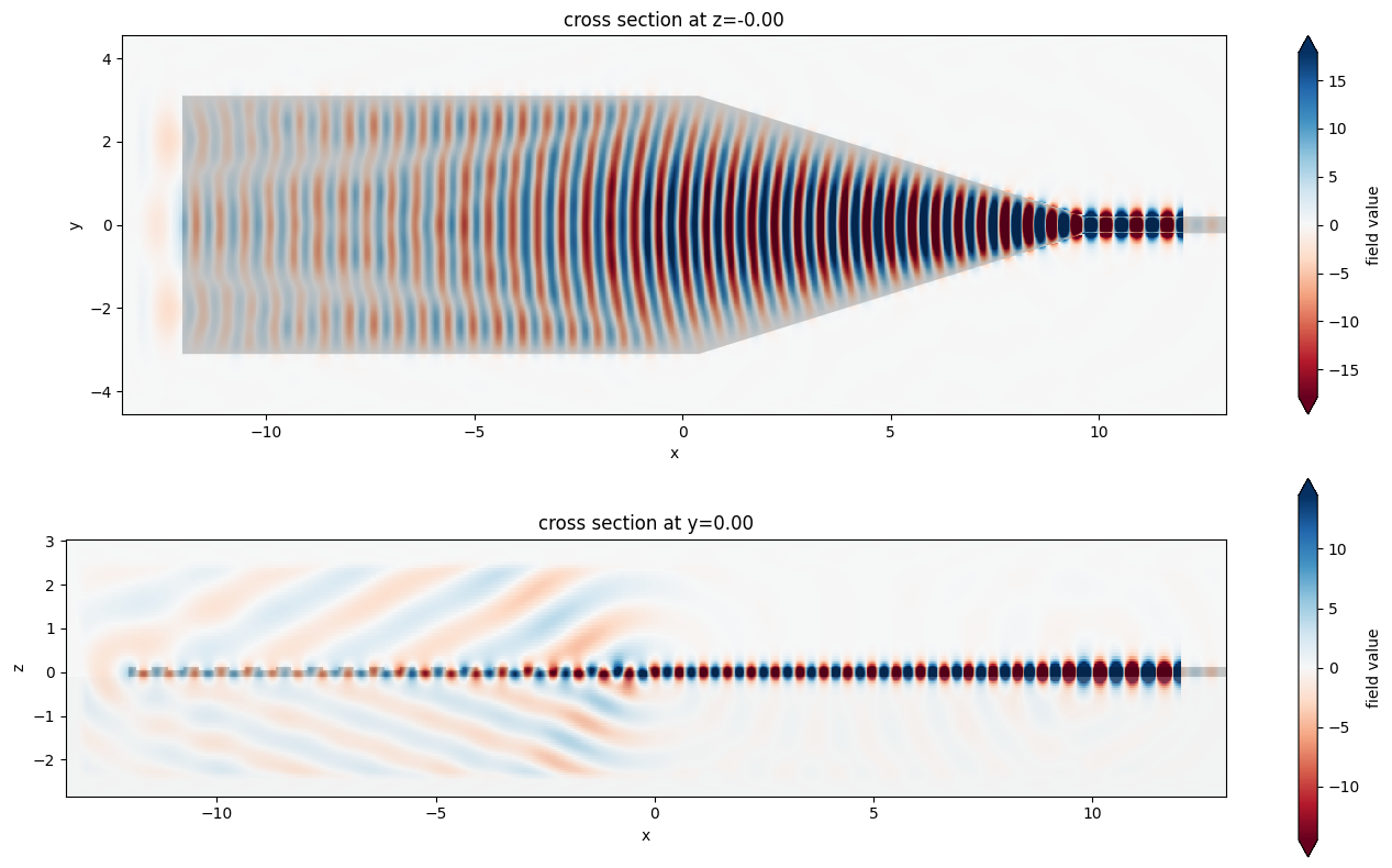
[16]:
fig, (ax1, ax2) = plt.subplots(2, 1, tight_layout=True, figsize=(14, 8))
sim_data.plot_field("full_domain_fields", "Ey", f=freq0, ax=ax1)
sim_data.plot_field("radiated_fields", "Ey", f=freq0, ax=ax2)
[16]:
<AxesSubplot: title={'center': 'cross section at y=0.00'}, xlabel='x', ylabel='z'>
Far Field Projection#
Now we use the Tidy3D’s FieldProjector to compute the anglular dependence of the far field scattering based on the near field monitor.
[17]:
# create range of angles to probe (note: polar coordinates, theta = 0 corresponds to vertical (z axis))
num_angles = 1101
thetas = np.linspace(-np.pi / 2, np.pi / 2, num_angles)

# make a near-to-far monitor specifying the observation angles and frequencies of interest
monitor_n2f = td.FieldProjectionAngleMonitor(
    center=near_field_monitor.center,
    size=near_field_monitor.size,
    normal_dir="+",
    freqs=[freq0],
    theta=thetas,
    phi=[0.0],
    name="n2f",
)

# make a near field to far field projector with the near field monitor data
near_field_surface = td.FieldProjectionSurface(
    monitor=near_field_monitor, normal_dir="+"
)
n2f = td.FieldProjector(sim_data=sim_data, surfaces=[near_field_surface])

# compute the far_fields
far_fields = n2f.project_fields(monitor_n2f)

# Compute the scattered cross section
Ps = far_fields.radar_cross_section.sel(f=freq0).values[0, ...]
[18]:
# plot the angle dependence
fig, ax = plt.subplots(subplot_kw={"projection": "polar"}, figsize=(5, 5))
ax.plot(thetas, np.abs(Ps), label="measured")
ax.plot(
    [design_theta_rad, design_theta_rad],
    [0, np.max(Ps) * 0.7],
    "r--",
    alpha=0.8,
    label="design angle",
)
ax.set_theta_zero_location("N")
ax.set_theta_direction(-1)
ax.set_yticklabels([])
ax.set_title("Scattered Cross-section (arb. units)", va="bottom")
plt.legend()
plt.show()
/Users/twhughes/.pyenv/versions/3.10.9/lib/python3.10/site-packages/matplotlib/cbook/__init__.py:1369: ComplexWarning: Casting complex values to real discards the imaginary part
  return np.asarray(x, float)
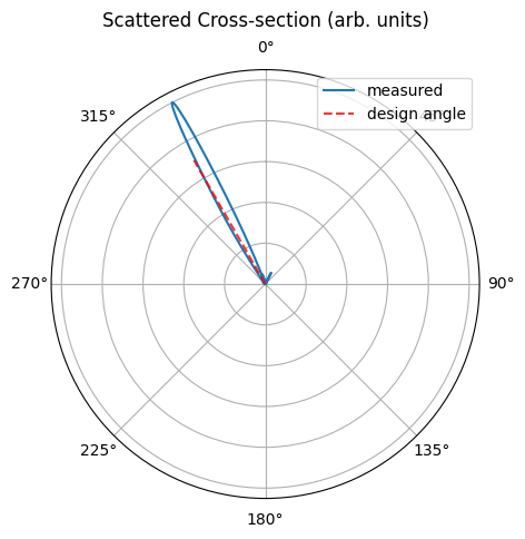
[19]:
print(f"expect angle of {(design_theta_rad * 180 / np.pi):.2f} degrees")
i_max = np.argmax(Ps)
print(f"got maximum angle of {(thetas[i_max] * 180 / np.pi):.2f} degrees")
expect angle of -30.00 degrees
got maximum angle of -27.16 degrees
The agreement between the target angle and the actual emission angle of the coupler is good. The small difference comes from the fact that the design is very sensitive to the value of the effective index that we use in the coupler region, and that value depends on which waveguide height we pick in that region: the one with the grating comb, or without. In our setup, we used a thickness that is at the mid-point, but this is a heuristic choice which results in the small final mismatch in angles observed here.
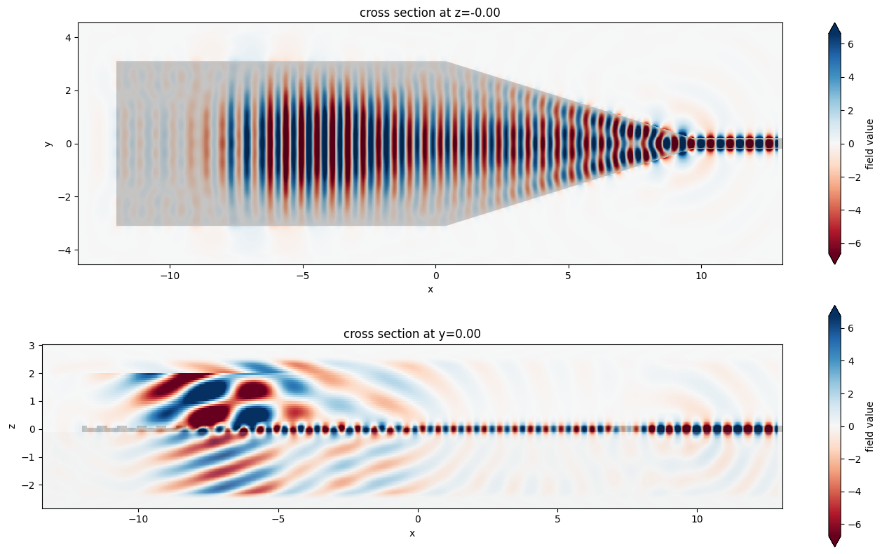
Gaussian beam into the coupler#
We can also run the coupler in the opposite way, injecting a Gaussian beam from above and monitoring the transmission into the waveguide. We will use the measured angle rather than the design angle to see the highest in-coupling efficiency that we can obtain.
[20]:
gaussian_beam = td.GaussianBeam(
    size=(td.inf, td.inf, 0),
    center=[-8, 0, 2],
    source_time=td.GaussianPulse(freq0=freq0, fwidth=fwidth),
    angle_theta=27.16 * np.pi / 180,
    angle_phi=np.pi,
    direction="-",
    waist_radius=2,
    pol_angle=np.pi / 2,
)

mode_mon = ms.to_monitor(freqs=[freq0], name="coupled")

flux_mon = td.FluxMonitor(
    size=mode_mon.size,
    center=mode_mon.center,
    freqs=[freq0],
    name="flux",
)


sim2 = td.Simulation(
    size=sim_size,
    grid_spec=grid_spec,
    structures=[sub, wg, cp, tp] + gratings,
    sources=[gaussian_beam],
    monitors=[plane_monitor, rad_monitor, mode_mon, flux_mon],
    run_time=run_time,
    boundary_spec=td.BoundarySpec.all_sides(boundary=td.PML()),
)
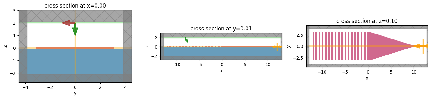
[21]:
fig, (ax1, ax2, ax3) = plt.subplots(1, 3, tight_layout=True, figsize=(14, 3))
sim2.plot(x=0, ax=ax1)
sim2.plot(y=0.01, ax=ax2)
sim2.plot(z=0.1, ax=ax3)
plt.show()
[22]:
job2 = web.Job(simulation=sim2, task_name="grating_coupler_beam")
sim_data2 = job2.run(path="data/grating_coupler.hdf5")
print(sim_data2.log)
Simulation domain Nx, Ny, Nz: [1157, 334, 102]
Applied symmetries: (0, 0, 0)
Number of computational grid points: 4.0500e+07.
Using subpixel averaging: True
Number of time steps: 1.3520e+05
Automatic shutoff factor: 1.00e-05
Time step (s): 3.8241e-17


Compute source modes time (s):     1.8071
Compute monitor modes time (s):    0.5088
Rest of setup time (s):            4.0165

Running solver for 135204 time steps...
- Time step   1076 / time 4.11e-14s (  0 % done), field decay: 1.00e+00
- Time step   5408 / time 2.07e-13s (  4 % done), field decay: 9.71e-03
- Time step  10816 / time 4.14e-13s (  8 % done), field decay: 1.60e-03
- Time step  16224 / time 6.20e-13s ( 12 % done), field decay: 2.77e-05
- Time step  21632 / time 8.27e-13s ( 16 % done), field decay: 5.87e-06
Field decay smaller than shutoff factor, exiting solver.

Solver time (s):                   57.9375
[23]:
fig, (ax1, ax2) = plt.subplots(2, 1, tight_layout=True, figsize=(14, 8))
sim_data2.plot_field("full_domain_fields", "Ey", f=freq0, ax=ax1)
sim_data2.plot_field("radiated_fields", "Ey", f=freq0, ax=ax2)
[23]:
<AxesSubplot: title={'center': 'cross section at y=0.00'}, xlabel='x', ylabel='z'>
[24]:
flux = sim_data2["flux"].flux
print(f"flux in waveguide / flux in = {float(flux):.4f} ")
flux in waveguide / flux in = 0.0485
The coupler has close to 5% in-coupling efficiency, and we did not put any effort into optimizing it beyond just defining the grating pitch to target the correct angle!