Frequently Asked Questions
Contents
Frequently Asked Questions#
How do I run a simulation and access the results?#
Submitting and monitoring jobs, and donwloading the results, is all done
through our web API. After a successful run,
all data for all monitors can be downloaded in a single .hdf5 file
using tidy3d.web.webapi.load(), and the
raw data can be loaded into a SimulationData object.
From the SimulationData object, one can grab and plot the data for each monitor with square bracket indexing, inspect the original Simulation object, and view the log from the solver run. For more details, see this tutorial.
How is using Tidy3D billed?#
The Tidy3D client that is used for designing
simulations and analyzing the results is free and
open source. We only bill the run time of the solver on our server, taking only the compute
time into account (as opposed to overhead e.g. during uploading).
When a task is uploaded to our servers, we will print the maximum incurred cost in Flex units.
This cost is also displayed in the online interface for that task.
This value is determined by the cost associated with simulating the entire time stepping specified.
If early shutoff is detected and the simulation completes before the full time stepping period, this
cost will be pro-rated.
For more questions or to purchase Flex units, please contact us at support@flexcompute.com.
What are the units used in the simulation?#
We assume the following physical units:
Length: micron (μm, \(10^{-6}\) meters)
Time: Second (s)
Frequency: Hertz (Hz)
Electric conductivity: Siemens per micron (S/μm)
Thus, the user should be careful, for example to use the speed of light
in μm/s when converting between wavelength and frequency. The built-in
speed of light td.C_0 has a unit of μm/s.
For example:
wavelength_um = 1.55
freq_Hz = td.C_0 / wavelength_um
wavelength_um = td.C_0 / freq_Hz
Currently, only linear evolution is supported, and so the output fields have an arbitrary normalization proportional to the amplitude of the current sources, which is also in arbitrary units. In the API Reference, the units are explicitly stated where applicable.
How do I add PML absorbing boundaries to my simulation?#
Upon initializing a simulation, the user can provide an optional argument pml_layers,
an array of three elements defining the PML boundaries along x, y, and z. The
easiest way to define PML is to use e.g. pml_layers=(None, None, td.PML())
to define PML in the z-direction only (in x and y, the default periodic boundaries will
be used). It is also possible to customize the PML further as explained in the
documentation and below.
Tidy3D uses a complex frequency-shifted formulation of the perfectly-matched layers (CPML),
for which it is more natural to define the thickness as number of layers rather than as
physical size. We provide two pre-set PML profiles, ‘standard’ (PML) and ‘stable’ (StablePML.
The standard profile has 12 layers by default and should be sufficient in many situations. In the
case of a diverging simulation, or when the fields do not appear to be fully absorbed in the PML,
the user can increase the number of layers in the ‘standard’ profile (PML(num_layers=20), or try the ‘stable’
profile, which requires more layers (default is 40) but should generally work better.
Adiabatic absorbing boundaries can be used as well through Absorber, which may improve stability over both PML types in certain situations.
NB: The PML layers extend beyond the simulation domain. This makes it easier not to worry
about PMLs intruding into parts of your simulation where you don’t want them to be. The one thing
to keep in mind, however, is that structures that span the full simulation should also extend into
the PML. So when defining such structures, it is best to extend them well beyond
the simulation size. You could even use td.inf, a shortcut for a very large value, for
dimensions that span the full domain. Below is an example of a right and a wrong way to make a
dielectric slab.
import tidy3d as td
import matplotlib.pyplot as plt

sim_size = [4., 4., 3.]
pml_layers = [td.PML(), td.PML(), td.PML()]

# Correct way: extend slab beyond simulation domain
slab_right = td.Structure(
    geometry=td.Box(
        center=[0, 0, 0],
        size=[td.inf, td.inf, .5],
    ),
    medium=td.Medium(epsilon=5)
)

sim_right = td.Simulation(
    size=sim_size,
    grid_size=0.05,
    structures=[slab_right],
    pml_layers=pml_layers)

# Wrong: use simulation domain size when using PML
slab_wrong = td.Structure(
    geometry=td.Box(
        center=[0, 0, 0],
        size=[sim_size[0], sim_size[1], .5],
    ),
    medium=td.Medium(epsilon=5)
)

sim_wrong = td.Simulation(
    size=sim_size,
    resolution=20,
    structures=[slab_wrong],
    pml_layers=pml_layers)

fig, ax = plt.subplots(1, 2, figsize=(11, 4))
sim_right.plot_eps(y=0, ax=ax[0])
sim_wrong.plot_eps(y=0, ax=ax[1])
ax[0].set_title('Right: extend through PML')
ax[1].set_title('Wrong: use simulation domain size')
plt.show()
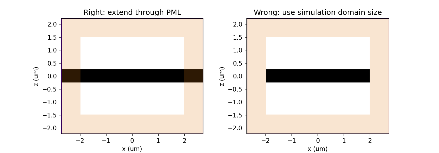
Notice that the simulation size in y is defined as 4 micron on initialization,
but the full simulation domain with the PML layers is 5.5 micron. A large number of PML
layers can thus lead to a significant increase of computation time in some cases.
Why is a simulation diverging?#
Sometimes, a simulation is numerically unstable and can result in divergence. The two things that can be tuned to avoid that are the thickness of the PML layers and the Courant stability factor, each of which are defined upon initializing a simulation. If materials with frequency-independent permittivity smaller than one are included in the simulation, the Courant factor must be set to a value lower than the lowest refractive index. In the case of dispersive materials, understanding the reason for the instability is a matter of trial and error. Some things to try include:
Remove dispersive materials extending into the PML.
Increase the number of PML layers.
Decrease the value of the Courant stability factor. Note that this leads to an inversely proportional increase in the simulation time.
How do I include material dispersion?#
Dispersive materials are supported in Tidy3D and we provide an extensive material library with pre-defined materials. Standard dispersive material models can also be defined. If you need help inputting a custom material, let us know!
It is important to keep in mind that dispersive materials are inevitably slower to
simulate than their dispersion-less counterparts, with complexity increasing with the
number of poles included in the dispersion model. For simulations with a narrow range
of frequencies of interest, it may sometimes be faster to define the material through
its real and imaginary refractive index at the center frequency. This can be done by
defining directly a value for the real part of the relative permittivity
\(\mathrm{Re}(\epsilon_r)\) and electric conductivity \(\sigma\) of a Medium,
or through a real part \(n\) and imaginary part \(k\). The relationship between the two equivalent models is
In the case of (almost) lossless dielectrics, the dispersion could be negligible in a broad frequency window, but generally, it is importat to keep in mind that such a material definition is best suited for single-frequency results.
For lossless, weakly dispersive materials, the best way to incorporate the dispersion
without doing complicated fits and without slowing the simulation down significantly is to
include the value of the refractive index dispersion \(\mathrm{d}n/\mathrm{d}\lambda\)
in units of 1/micron when defining the Medium. The value is assumed to be
at the central frequency or wavelength (whichever is provided), and a one-pole model for the
material is generated. These values are for example readily available from the
refractive index database.
Why can I not change Tidy3D instances after they are created?#
You may notice in Tidy3D verions 1.5 and above that it is no longer possible to modify instances of Tidy3D components after they are created. Making Tidy3D components immutable like this was an intentional design decision indended to make Tidy3D safer and more performant.
For example, Tidy3D contains several “validators” on input data. If models are mutated, we can’t always guarantee that the resulting instance will still satisfy our validations and the simulation may be invalid.
Furthermore, making the objects immutable allows us to cache the results of many expensive operations. For example, we can now compute and store the simulation grid once, without needing to worry about the value becoming stale at a later time, which significantly speeds up plotting and other operations.
If you have a Tidy3D component that you want to recreate with a new set of parameters, instead of obj.param1 = param1_new, you can call obj_new = obj.copy(update=dict(param1=param1_new)).
Note that you may also pass more key value pairs to the dictionary in update.