Run CFD using Python API: An example of ONERA M6 Wing
Contents
1.2. Run CFD using Python API: An example of ONERA M6 Wing#
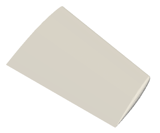
The Onera M6 wing is a classic CFD validation case for external flows because of its simple geometry combined with complexities of transonic flow (i.e. local supersonic flow, shocks, and turbulent boundary layer separation). It is a swept, semi-span wing with no twist and uses a symmetric airfoil using the ONERA D section. More information about the geometry can be found at NASA’s website. The geometry parameters of the model are:
Mean Aerodynamic Chord (MAC) = 0.80167 m
Semi-span = 1.47602 m
Reference area = 1.15315 m2
The mesh used for this case contains 113K nodes and 663K tetrahedrons, and the flow conditions are:
Mach Number = 0.84
Reynolds Number (based on MAC) = 11.72 Million
Alpha = 3.06°
Reference Temperature = 297.78 K
1.2.1. Upload the Mesh File#
Before uploading a mesh, if you have not done so already, install the Flow360 Python API client. For installation instructions, visit the API Reference section of this documentation. To upload a mesh and run a case, open your Python interpreter and import the flow360 client.
python3
import flow360client
Specify no-slip boundaries - you can do this in three ways:
By directly feeding it into the noSlipWalls argument:
noSlipWalls = [1]
By using the .mapbc file:
noSlipWalls = flow360client.noSlipWallsFromMapbc('/path/to/fname.mapbc')
(Note: Make sure the boundary names in your .mapbc file do NOT contain any spaces )
And by using the meshJson object:
import json
meshJson = json.load(open('/path/to/Flow360Mesh.json'))
The Flow360Mesh.json file for this tutorial has the following contents:
{
    "boundaries" :
    {
     "noSlipWalls" : [1]
    }
}
Download the mesh file from here. If using options (a) and (b), use the following command to upload your mesh:
meshId = flow360client.NewMesh(fname='/path/to/mesh.lb8.ugrid',
                               noSlipWalls=noSlipWalls,
                               meshName='my_mesh',
                               tags=[],
                               endianness='little'
                              )
If using option (c), use the following command to upload your mesh:
meshId = flow360client.NewMesh(fname='/path/to/mesh.lb8.ugrid',
                               meshJson=meshJson,
                               meshName='my_mesh',
                               tags=[],
                               endianness='little'
                              )
(Note: Arguments of meshName and tags are optional. If using a mesh filename of the format mesh.lb8.ugrid (little-endian format) or mesh.b8.ugrid (big-endian format), the endianness argument is optional. However, if you choose to use a mesh filename of the format mesh.ugrid, you must specify the appropriate endianness (‘little’ or ‘big’) in NewMesh. More information on endianness can be found here.)
Currently supported mesh file formats are .ugrid, .cgns and their .gz and .bz2 compressions. The mesh status can be checked by using:
## to list all your mesh files
flow360client.mesh.ListMeshes()
## to view a particular mesh
flow360client.mesh.GetMeshInfo('mesh_Id')
Replace the mesh_Id with your mesh’s ID.
1.2.2. Run a Case#
The Flow360.json file for this case has the following contents. A full dictionary of configuration parameters for the JSON input file can be found here.
 1{
 2    "geometry" : {
 3        "meshName" : "wing_tetra.1.lb8.ugrid",
 4        "refArea" : 1.15315084119231,
 5        "momentCenter" : [0.0, 0.0, 0.0],
 6        "momentLength" : [1.47602, 0.801672958512342, 1.47602]
 7    },
 8        "volumeOutput" : {
 9        "outputFormat" : "tecplot",
10        "animationFrequency" : -1,
11        "primitiveVars" : true,
12        "vorticity" : false,
13        "residualNavierStokes" : false,
14        "residualTurbulence" : false,
15        "T" : false,
16        "s" : false,
17        "Cp" : false,
18        "mut" : false,
19        "mutRatio" : false,
20        "Mach" : true
21    },
22    "surfaceOutput" : {
23        "outputFormat" : "tecplot",
24        "animationFrequency" : -1,
25        "primitiveVars" : true,
26        "Cp" : true,
27        "Cf" : true,
28        "CfVec" : false,
29        "yPlus" : false,
30        "wallDistance" : false
31    },
32    "sliceOutput" : {
33        "outputFormat" : "tecplot",
34        "animationFrequency" : -1,
35            "primitiveVars" : true,
36            "vorticity" : true,
37            "T" : true,
38            "s" : true,
39            "Cp" : true,
40            "mut" : true,
41            "mutRatio" : true,
42            "Mach" : true
43        },
44    "navierStokesSolver" : {
45        "absoluteTolerance" : 1e-10,
46        "kappaMUSCL" : -1.0
47    },
48    "turbulenceModelSolver" : {
49        "modelType" : "SpalartAllmaras",
50        "absoluteTolerance" : 1e-8,
51        "kappaMUSCL" : -1.0
52    },
53    "freestream" :
54    {
55        "Reynolds" : 14.6e6,
56        "Mach" : 0.84,
57        "Temperature" : 288.15,
58        "alphaAngle" : 3.06,
59        "betaAngle" : 0.0
60    },
61    "boundaries" : {
62        "1" : {
63            "type" : "NoSlipWall",
64            "name" : "wing"
65        },
66        "2" : {
67            "type" : "SlipWall",
68            "name" : "symmetry"
69        },
70        "3" : {
71            "type" : "Freestream",
72            "name" : "freestream"
73        }
74    },
75    "timeStepping" : {
76        "maxPseudoSteps" : 500,
77        "CFL" : {
78            "initial" : 5,
79            "final": 200,
80            "rampSteps" : 40
81        }
82    }
83}
Use this JSON configuration file and run the case with the following command:
caseId = flow360client.NewCase(meshId='mesh_Id',
                               config='/output/path/for/Flow360.json',
                               caseName='my_case',
                               tags=[]
                              )
(Note: Arguments of meshName and tags are optional.)
The case status can be checked by using:
## to list all your cases
flow360client.case.ListCases()
## to view a particular case
flow360client.case.GetCaseInfo('case_Id')
Replace the mesh_Id and case_Id with your mesh and case IDs, respectively.
1.2.3. Deleting a Mesh/Case#
An uploaded mesh/case can be deleted using the following commands (Caution: You will not be able to recover your deleted case or mesh files including its results after your deletion):
## Delete a mesh
flow360client.mesh.DeleteMesh('')
## Delete a case
flow360client.case.DeleteCase('')
1.2.4. Download the Results#
To download the surface data (surface distributions and slices) and the entire flow field, use the following command lines, respectively:
flow360client.case.DownloadSurfaceResults('case_Id', 'surfaces.tar.gz')
flow360client.case.DownloadVolumetricResults('case_Id', 'volume.tar.gz')
Once downloaded, you can postprocess these output files in either Tecplot or ParaView. You can specify this in the Flow360.json file under the volumeOutput, surfaceOutput, and sliceOutput sections.
To download the solver.out file, use the following command:
flow360client.case.DownloadSolverOut('case_Id', fileName='flow360_case.user.log')
You can also download the nonlinear residuals, surface forces and total forces by using the following command line:
flow360client.case.DownloadResultsFile('case_Id', 'fileName.csv')
Replace caseId with your caseId and fileName with nonlinear_residual, surface_forces and total_forces for their respective data.
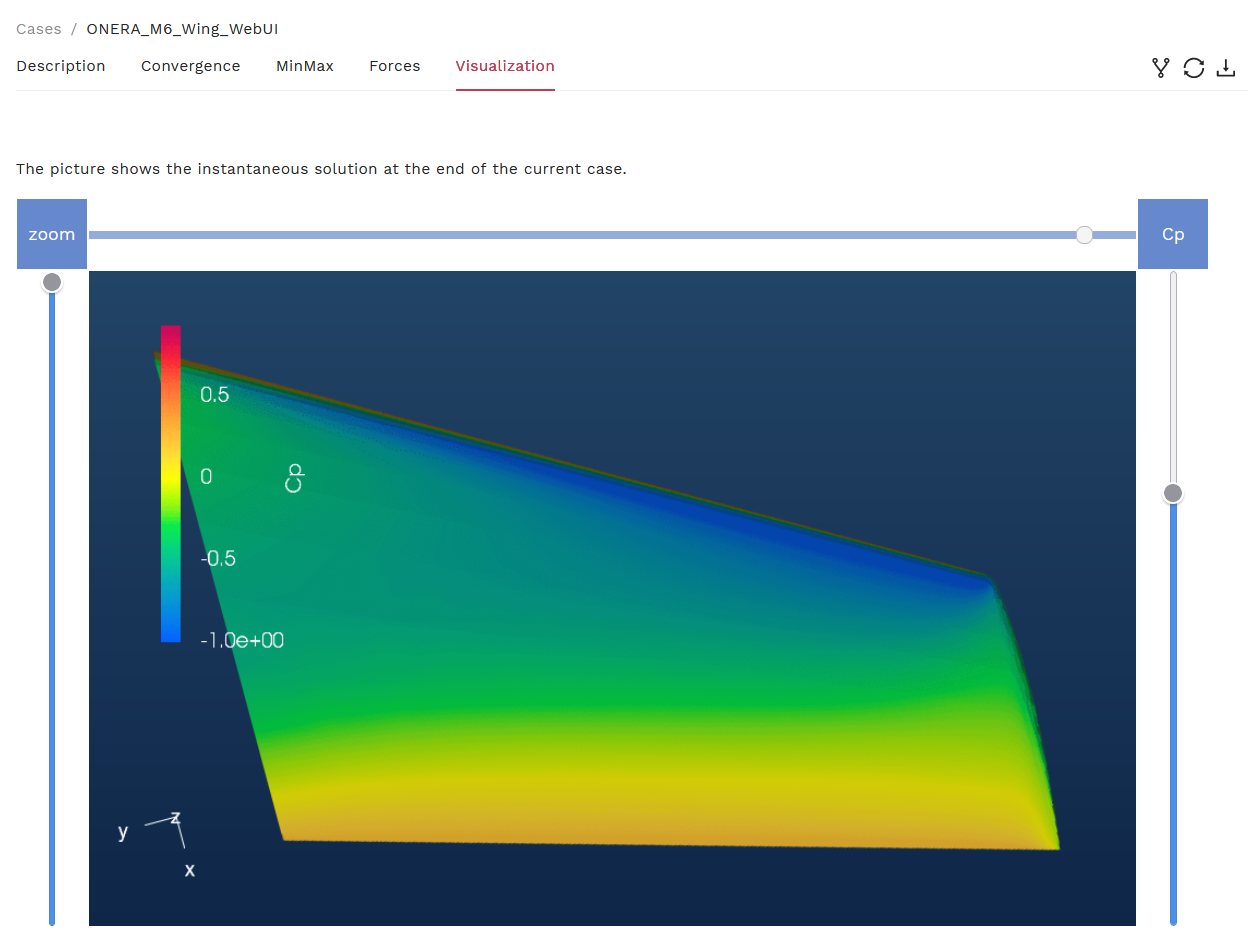
1.2.5. Visualizing the Results#
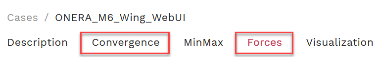
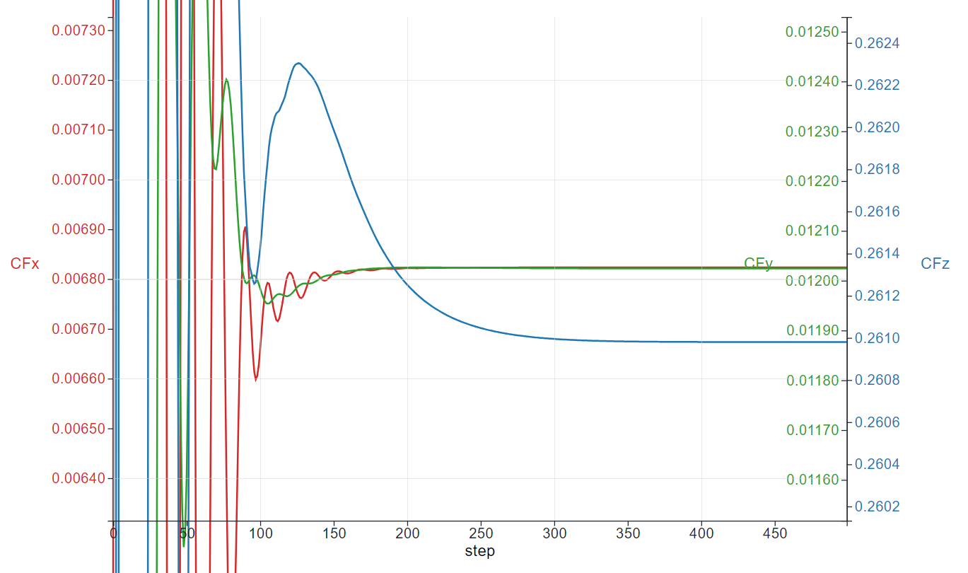
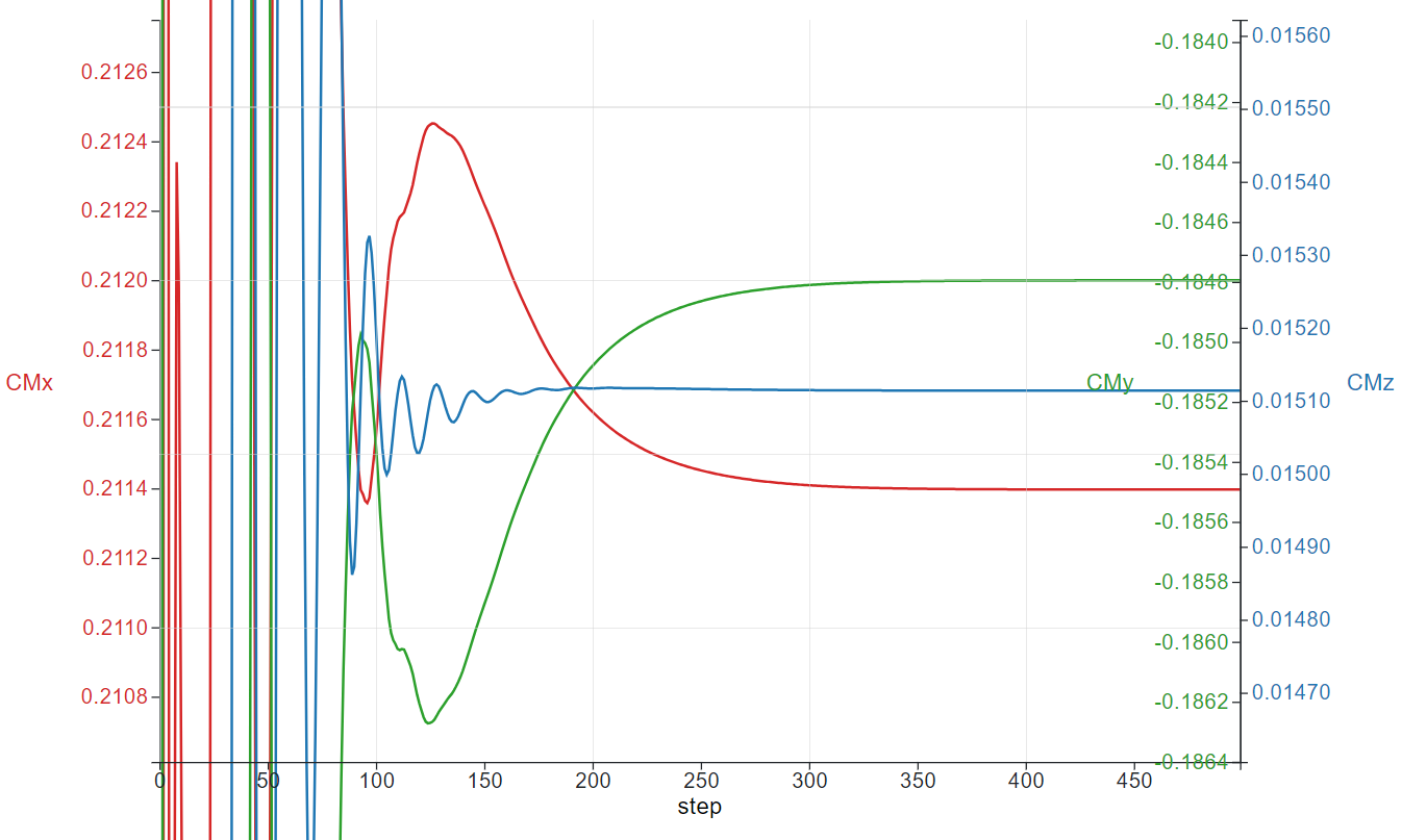
While your case is running, or after that, you can visualize the Residuals and Forces plot on our website (https://client.flexcompute.com/app/case/all) by clicking on your case name and viewing them under the Convergence and Forces tabs, respectively.
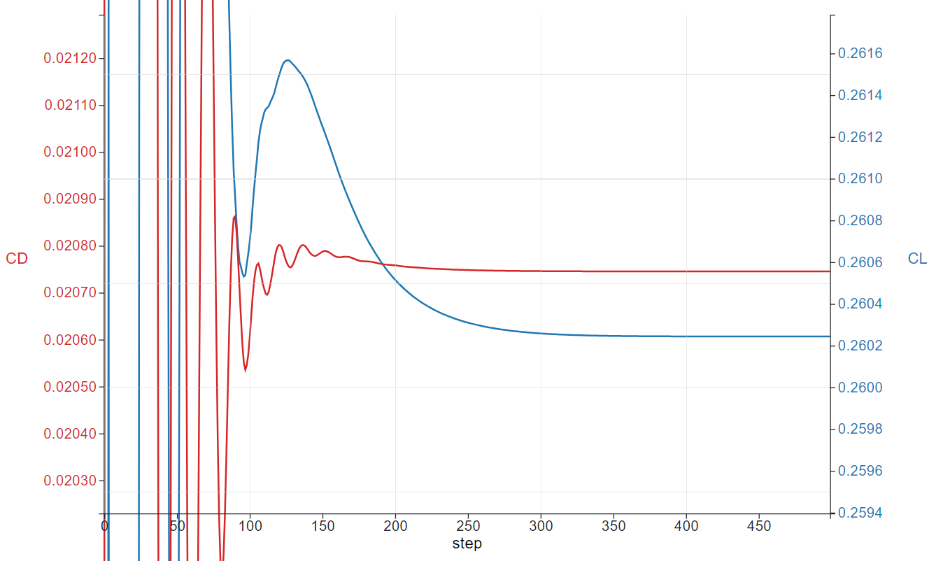
For example, the Forces plots for this case are:
Once your case has completed running, you can also visualize the contour plots of the results under the Visualization tab. Currently, contour plots for Coefficient of Pressure (Cp), Coefficient of Skin Friction (Cf), y+, and Cf with streamlines are provided.