2.4. User Defined Dynamics

In Flow360, users are now able to specify arbitrary dynamics. In what follows, an example for a Proportional-Integral (PI) controller and an example for Aero-Structural Interaction (ASI) are given.

2.4.1. PI controller for angle of attack to control lift coefficient

In this example, we add a controller to om6Wing case study. Based on the entries of the configuration file in this case study, the resulting value of the lift coefficient, CL, obtained from the simulation is ~0.26. Our objective is to add a controller to this case study such that for a given target value of CL (e.g., 0.4), the required angle of attack, alphaAngle , is estimated. To this end, a PI controller is defined under userDefinedDynamics in the configuration file as:

"userDefinedDynamics": [
    {
        "dynamicsName": "alphaController",
        "inputVars": [
            "CL"
        ],
        "constants": {
            "CLTarget": 0.4,
            "Kp": 0.2,
            "Ki": 0.002
        },
        "outputVars": {
            "alphaAngle": "if (pseudoStep > 500) state[0]; else alphaAngle;"
        },
        "stateVarsInitialValue": [
            "alphaAngle",
            "0.0"
        ],
        "updateLaw": [
            "if (pseudoStep > 500) state[0] + Kp * (CLTarget - CL) + Ki * state[1]; else state[0];",
            "if (pseudoStep > 500) state[1] + (CLTarget - CL); else state[1];"
        ],
        "inputBoundaryPatches": [
            "1"
        ]
    }
]

The complete case configuration file can be downloaded here: Flow360.json.

Some of the parameters are dicussed in more detail here:

1. dynamicsName: This is a name selected by the user for the dynamics. The results of user-defined dynamics are saved to udd_dynamicsName_v2.csv.

2. constants: This includes a list of all the constants related to this dynamics. These constants will be used in the equations for updateLaw and outputVars. In the above-mentioned example, CLTarget, Kp, and Ki are the target value of the lift coefficient, the proportional gain of the controller, and the integral gain of the controller, respectively.

3. outputVars: Each outputVars consists of the variable name and the relations between the variable and the state variables. For this example, we set the output variable equal to the angle of attack calculated by the controller after the first 500 pseudoSteps (i.e., state[0]).

4. stateVarsInitialValue: There are two state variables for this controller. The first one, state[0], is the angle of attack computed by the controller, and the second one, state[1], is the summation of error (CLTarget - CL) over iterations. The initial values of state[0] and state[1] are set to alphaAngle and 0, respectively.

5. updateLaw: The expressions for the state variables are specified here. The first and the second expressions correspond to equations for state[0] and state[1], respectively. The conditional statement forces the controller not to be run for the first 500 pseudoSteps. This ensures that the flow field is established to some extent before the controller is initialized.

6. inputBoundaryPatches: The related boundary conditions for the inputs of the user-defined dynamics are specified here. In this example, the noSlipWall boundary conditions are where CL is calcualted. As seen in the configuration file, the boundary name for the No-Slip boundary condition is "1".

The following figure shows the values of lift coefficient, CL, and angle of attack, alphaAngle, versus the steps, pseudoStep. As specified in the configuration file, the initial value of angle of attack is 3.06. With the specified user-defined dynamics, alphaAngle is adjusted to a final value of 4.61 so that CL = 0.4 is achieved.

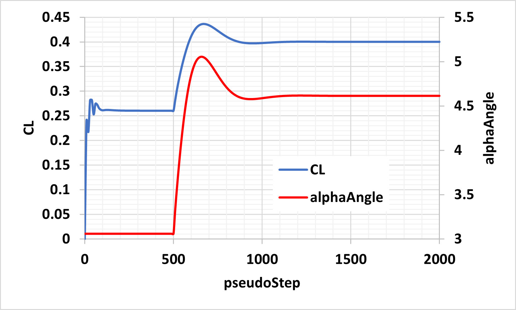
Fig. 2.4.1 Results of alphaController for om6Wing case study.

2.4.2. Dynamic grid rotation using structural aerodynamic load

In this example, we present an illustrative case where a flat plate rotates while being subjected to a rotational spring moment and damper as well as aerodynamic loads. Below is a video showing the flutter motion of the plate.

Fig. 2.4.2 Flutter motion of the plate under aerodynamic and structural forces.

The userDefinedDynamics section of the case JSON is presented below:

{
    "userDefinedDynamics": [
        {
            "dynamicsName": "dynamicTheta",
            "inputVars": [
                "rotMomentY"
            ],
            "constants": {
                "I": 0.443768309310345,
                "zeta": 4.0,
                "K": 0.0161227107,
                "omegaN": 0.190607889,
                "theta0": 0.0872664626
            },
            "outputVars": {
                "omegaDot[plate]": "state[0];",
                "omega[plate]": "state[1];",
                "theta[plate]": "state[2];"
            },
            "stateVarsInitialValue": [
                "0.0",
                "0.0",
                "1.39626340e-01"
            ],
            "updateLaw": [
                "if (pseudoStep == 0) (rotMomentY - K * ( state[2] - theta0 ) - 2 * zeta * omegaN * I *state[1] ) / I; else state[0];",
                "if (pseudoStep == 0) state[1] + state[0] * timeStepSize; else state[1];",
                "if (pseudoStep == 0) state[2] + state[1] * timeStepSize; else state[2];"
            ],
            "inputBoundaryPatches": [
                "plateBlock/noSlipWall"
            ]
        }
    ]
}

The complete case configuration file can be downloaded here: Flow360.json.

For this case the dynamics of the plate is:

(2.4.1)\[\ddot{\theta} = \left[ \tau_y - K \cdot \left( \theta-\theta_0 \right) - 2\zeta\omega_N I \dot{\theta} \right]/I\]

(2.4.2)\[\dot{\theta} -\dot{\theta}_0= \int_{0}^{t} \ddot{\theta}\left(t'\right) \, dt'\]

(2.4.3)\[\theta -\theta_0 = \int_{0}^{t} \dot{\theta}\left(t'\right) \, dt'\]

which cooresponds to the three updateLaw shown above. Below is a table for the symbols and their respective physical meannings:

Symbol	Description
\(\theta\)	Rotation angle of the plate in radius.
\(\tau_y\)	Aerodynamic moment exerted on the plate.
\(K\)	Stiffness of the spring attached to the plate at the structural support.
\(\zeta\)	Structural damping ratio.
\(\omega_N\)	Structural natural angular frequency.
\(I\)	Structural moment of inertia.

In the inputVars, the rotMomentY is the Y component of the rotational moment by the aerodynamic force. The moment is calculated around momentCenter.

Note that OutputVars follows the format of VarName[slidingInterfaceName] : Relation to state variable. In this case the name of sliding interface is plate. \(\ddot{\theta}\), \(\dot{\theta}\), \(\theta\), are assigned as the first, second and third state variables, respectively.