1.4. Run CFD using Automated Meshing and Python API

For this quick start on Automated Meshing with the Python API, we will once again use the ONERA M6 Wing case. We will show you how to submit a *.csm geometry file using the Python API and run a simulation.

The geometry model is built in Engineering Sketch Pad (ESP). More information about ESP installation is available here. The ONERA M6 Wing Model in ESP can be found in the om6wing.csm file.

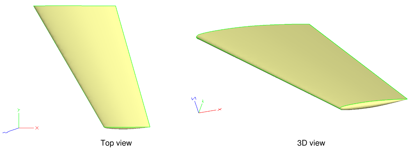
Fig. 1.4.1 ONERA M6 Wing generated in ESP

Through ESP we have control over the meshing parameters applied including edge and face attributes. The surface mesh parameters used here are available in the om6SurfaceMesh.json file.

Within the volume mesh parameters JSON file below, you will notice that we use field constraints to control the maximum edge length and resolution of the unstructured mesh. Similarly, the initial height of the anisotropic mesh at wall boundaries is indicated by ‘firstLayerThickness’ and ‘growthRate’.

The volume mesh parameters are available in the om6VolumeMesh.json file.

1.4.1. Case Setup

Flow conditions:

• Reynolds: 14.6e+6

• Mach: 0.84

• AoA: 3.06°

The case setup parameters for the ONERA M6 Wing simulation are available in the om6Case.json file.

1.4.2. Run a Case

Just like we did for the Web UI, through the Python API, first we generate the surface mesh from the CSM file, then the volume mesh is generated and finally we run the simulation. Please note that all the mesh generation happens on our servers. All you have to do is provide the appropriate input CSM and JSON files.

Using the Python API, these three steps are executed using the following commands:

surfaceMeshId = flow360client.NewSurfaceMeshFromGeometry("om6wing.csm", "om6SurfaceMesh.json")
volumeMeshId = flow360client.NewMeshFromSurface(surfaceMeshId=surfaceMeshId, config="om6VolumeMesh.json")
caseId = flow360client.NewCase(meshId = volumeMeshId, config="om6Case.json", caseName='QuickStart_OM6_AutomaticMeshing')

To ease the simulation process, an example Python script is provided here that takes a CSM, mesh and case input JSON files as the input configuration parameters for the simulation, submitCase.py. The input JSON file has the following content:

{
    "geometry": {
        "csm": "path/to/modelFile.csm"
    },
    "mesh": {
        "surface": "path/to/SurfaceMesh.json",
        "volume": "path/to/VolumeMesh.json"
    },
    "flow360": {
        "case": "path/to/simulationCase.json"
    }
}

To utilize, copy the content above into a JSON file called ‘simConfiguration.json’, then modify the individual paths for the *.csm file, surface and volume mesh JSON, and finally the case JSON files. Then submit using:

python3 submitCase.py -json simConfiguration.json

1.4.3. Download the Results

To download the surface and volume solution for postprocessing, we will also use the Flow360 Python API client.

The example script, downloadCase.py, takes a JSON input and downloads flow results as well as forces and moments convergence history files. The input JSON file has the following form:

{
    "flow360": {
        "caseId": "case_id",
        "caseName": "CaseName_QuickStartSimulation"
    }
}

To utilize, copy the content above into a JSON file called ‘getCase.json’. Then run ‘downloadCase.py’ to download the results.

python3 downloadCase.py -json getCase.json

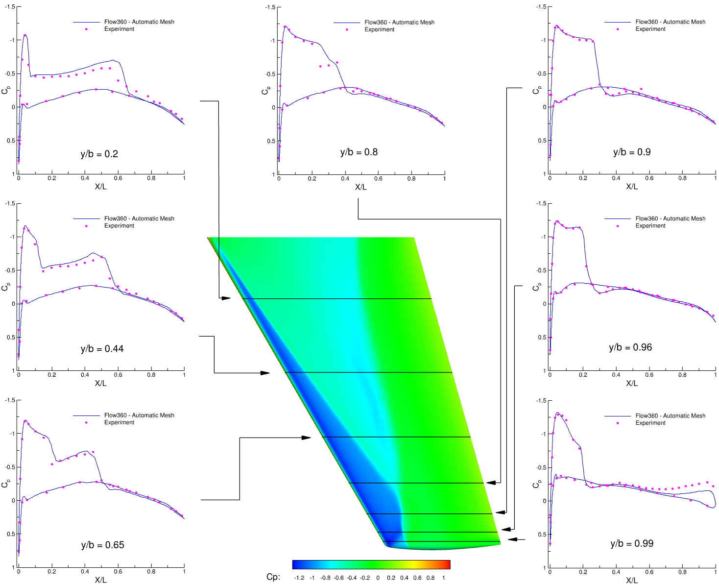
You can then postprocess results with either Tecplot or Paraview (output format is specified in the om6Case.json input file). Below you can find pressure coefficient comparisons with experimental data.

1.4.4. Visualize Force Histories

You can also find the force convergence histories on the Web UI by clicking on your case name and selecting the Forces tab.

For the ONERA M6 Wing simulation, the convergence histories of forces are:

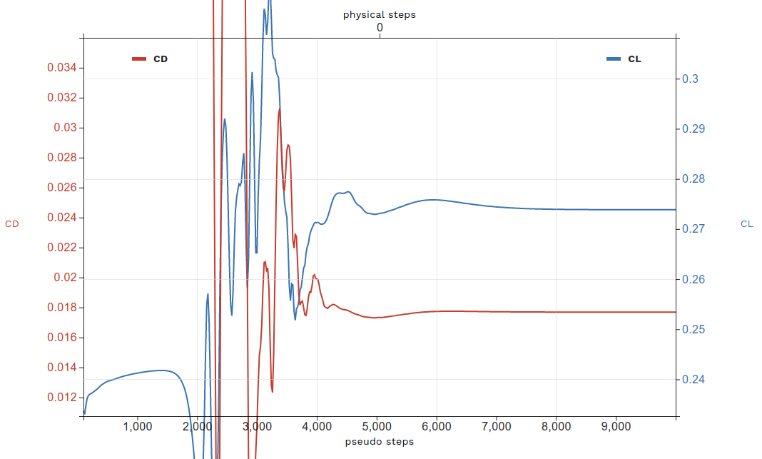
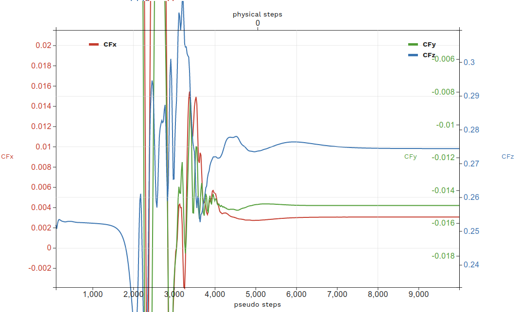
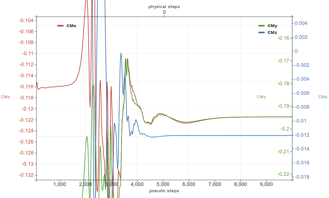
Alternatively, the force convergence histories are were downloaded through the Python API above to the total_forces_v2.csv file. The same force convergence histories can be plotted from total_forces_v2.csv.