tidy3d.EMESimulation#
- class EMESimulation[source]#
Bases:
AbstractYeeGridSimulationEigenMode Expansion (EME) simulation.
- Parameters:
attrs (dict = {}) – Dictionary storing arbitrary metadata for a Tidy3D object. This dictionary can be freely used by the user for storing data without affecting the operation of Tidy3D as it is not used internally. Note that, unlike regular Tidy3D fields,
attrsare mutable. For example, the following is allowed for setting anattrobj.attrs['foo'] = bar. Also note that Tidy3D` will raise aTypeErrorifattrscontain objects that can not be serialized. One can check ifattrsare serializable by callingobj.json().center (Tuple[float, float, float] = (0.0, 0.0, 0.0)) – [units = um]. Center of object in x, y, and z.
size (Tuple[NonNegativeFloat, NonNegativeFloat, NonNegativeFloat]) – [units = um]. Size in x, y, and z directions.
medium (Union[Medium, AnisotropicMedium, PECMedium, PoleResidue, Sellmeier, Lorentz, Debye, Drude, FullyAnisotropicMedium, CustomMedium, CustomPoleResidue, CustomSellmeier, CustomLorentz, CustomDebye, CustomDrude, CustomAnisotropicMedium, PerturbationMedium, PerturbationPoleResidue] = Medium(attrs={}, name=None, frequency_range=None, allow_gain=False, nonlinear_spec=None, modulation_spec=None, heat_spec=None, type='Medium', permittivity=1.0, conductivity=0.0)) – Background medium of simulation, defaults to vacuum if not specified.
structures (Tuple[Structure, ...] = ()) – Tuple of structures present in simulation. Note: Structures defined later in this list override the simulation material properties in regions of spatial overlap.
symmetry (Tuple[Literal[0, -1, 1], Literal[0, -1, 1], Literal[0, -1, 1]] = (0, 0, 0)) – Tuple of integers defining reflection symmetry across a plane bisecting the simulation domain normal to the x-, y-, and z-axis at the simulation center of each axis, respectively.
sources (Tuple[NoneType, ...] = ()) – Sources in the simulation. NOTE: sources are not currently supported for EME simulations. Instead, the simulation performs full bidirectional propagation in the ‘port_mode’ basis. After running the simulation, use ‘smatrix_in_basis’ to use another set of modes or input field.
boundary_spec (BoundarySpec = BoundarySpec(attrs={}, x=Boundary(attrs={},, plus=PECBoundary(attrs={},, name=None,, type='PECBoundary'),, minus=PECBoundary(attrs={},, name=None,, type='PECBoundary'),, type='Boundary'), y=Boundary(attrs={},, plus=PECBoundary(attrs={},, name=None,, type='PECBoundary'),, minus=PECBoundary(attrs={},, name=None,, type='PECBoundary'),, type='Boundary'), z=Boundary(attrs={},, plus=PECBoundary(attrs={},, name=None,, type='PECBoundary'),, minus=PECBoundary(attrs={},, name=None,, type='PECBoundary'),, type='Boundary'), type='BoundarySpec')) – Specification of boundary conditions along each dimension. If
None, PML boundary conditions are applied on all sides. NOTE: for EME simulations, this is required to be PECBoundary on all sides. To capture radiative effects, move the boundary farther away from the waveguide in the tangential directions, and increase the number of modes. The ‘ModeSpec’ can also be used to try different boundary conditions.monitors (Tuple[Annotated[Union[tidy3d.components.eme.monitor.EMEModeSolverMonitor, tidy3d.components.eme.monitor.EMEFieldMonitor, tidy3d.components.eme.monitor.EMECoefficientMonitor, tidy3d.components.monitor.ModeSolverMonitor], FieldInfo(default=PydanticUndefined, discriminator='type', extra={})], ...] = ()) – Tuple of monitors in the simulation. Note: monitor names are used to access data after simulation is run.
grid_spec (GridSpec = GridSpec(attrs={}, grid_x=AutoGrid(attrs={},, type='AutoGrid',, min_steps_per_wvl=10.0,, max_scale=1.4,, dl_min=0.0,, mesher=GradedMesher(attrs={},, type='GradedMesher')), grid_y=AutoGrid(attrs={},, type='AutoGrid',, min_steps_per_wvl=10.0,, max_scale=1.4,, dl_min=0.0,, mesher=GradedMesher(attrs={},, type='GradedMesher')), grid_z=AutoGrid(attrs={},, type='AutoGrid',, min_steps_per_wvl=10.0,, max_scale=1.4,, dl_min=0.0,, mesher=GradedMesher(attrs={},, type='GradedMesher')), wavelength=None, override_structures=(), type='GridSpec')) – Specifications for the simulation grid along each of the three directions. This is distinct from ‘eme_grid_spec’, which defines the 1D EME grid in the propagation direction.
version (str = 2.7.0rc2) – String specifying the front end version number.
lumped_elements (Tuple[LumpedResistor, ...] = ()) – Tuple of lumped elements in the simulation. Note: only
tidy3d.LumpedResistoris supported currently.subpixel (bool = True) – If
True, uses subpixel averaging of the permittivity based on structure definition, resulting in much higher accuracy for a given grid size.freqs (List[PositiveFloat]) – Frequencies for the EME simulation.
axis (Literal[0, 1, 2]) – Propagation axis (0, 1, or 2) for the EME simulation.
eme_grid_spec (Union[EMEUniformGrid, EMECompositeGrid, EMEExplicitGrid]) – Specification for the EME propagation grid. The simulation is divided into cells in the propagation direction; this parameter specifies the layout of those cells. Mode solving is performed in each cell, and then propagation between cells is performed to determine the complete solution. This is distinct from ‘grid_spec’, which defines the grid in the two tangential directions, as well as the grid used for field monitors.
store_port_modes (bool = True) – Whether to store the modes associated with the two ports. Required to find scattering matrix in basis besides the computational basis.
port_offsets (Tuple[NonNegativeFloat, NonNegativeFloat] = (0, 0)) – Offsets for the two ports, relative to the simulation bounds along the propagation axis.
sweep_spec (Union[EMELengthSweep, EMEModeSweep, NoneType] = None) – Specification for a parameter sweep to be performed during the EME propagation step. The results are stored in ‘sim_data.smatrix’. Other simulation monitor data is not included in the sweep.
constraint (Optional[Literal['passive', 'unitary']] = passive) – Constraint for EME propagation, imposed at cell interfaces. A constraint of ‘passive’ means that energy can be dissipated but not created at interfaces. A constraint of ‘unitary’ means that energy is conserved at interfaces (but not necessarily within cells). The option ‘none’ may be faster for a large number of modes. The option ‘passive’ can serve as regularization for the field continuity requirement and give more physical results.
Notes
EME is a frequency-domain method for propagating the electromagnetic field along a specified axis. The method is well-suited for propagation of guided waves. The electromagnetic fields are expanded locally in the basis of eigenmodes of the waveguide; they are then propagated by imposing continuity conditions in this basis.
The EME simulation is performed along the propagation axis
axisat frequenciesfreqs. The simulation is divided into cells along the propagation axis, as defined byeme_grid_spec. Mode solving is performed at cell centers, and boundary conditions are imposed between cells. The EME ports are defined to be the boundaries of the first and last cell in the EME grid. These can be moved usingport_offsets.An EME simulation always computes the full scattering matrix of the structure. Additional data can be recorded by adding ‘monitors’ to the simulation.
Other Bases
By default, the scattering matrix is expressed in the basis of EME modes at the two ports. It is sometimes useful to use alternative bases. For example, in a waveguide splitter, we might want the scattering matrix in the basis of modes of the individual waveguides. The functions smatrix_in_basis and field_in_basis in
EMESimulationDatacan be used for this purpose after the simulation has been run.Frequency Sweeps
Frequency sweeps are supported by including multiple frequencies in the freqs field. However, our EME solver repeats the mode solving for each new frequency, so frequency sweeps involving a large number of frequencies can be slow and expensive. If a large number of frequencies are required, consider using our FDTD solver instead.
Passivity and Unitarity Constraints
Passivity and unitarity constraints can be imposed via the constraint field. These constraints are imposed at interfaces between cells, possibly at the expense of field continuity. Passivity means that the interface can only dissipate energy, and unitarity means the interface will conserve energy (energy may still be dissipated inside cells when the propagation constant is complex). Adding constraints can slow down the simulation significantly, especially for a large number of modes (more than 30 or 40).
Too Many Modes
It is important to use enough modes to capture the physics of the device and to ensure that the results have converged (see below). However, using too many modes can slow down the simulation and result in numerical issues. If too many modes are used, it is common to see a warning about invalid modes in the simulation log. While these modes are not included in the EME propagation, this can indicate some other issue with the setup, especially if the results have not converged. In this case, extending the simulation size in the transverse directions and increasing the grid resolution may help by creating more valid modes that can be used in convergence testing.
Mode Convergence Sweeps
It is a good idea to check that the number of modes is large enough by running a mode convergence sweep. This can be done using
EMEModeSweep.Example
>>> from tidy3d import Box, Medium, Structure, C_0, inf
>>> from tidy3d import EMEModeSpec, EMEUniformGrid, GridSpec
>>> from tidy3d import EMEFieldMonitor
>>> lambda0 = 1
>>> freq0 = C_0 / lambda0
>>> sim_size = 3*lambda0, 3*lambda0, 3*lambda0
>>> waveguide_size = (lambda0/2, lambda0, inf)
>>> waveguide = Structure(
...     geometry=Box(center=(0,0,0), size=waveguide_size),
...     medium=Medium(permittivity=2)
... )
>>> eme_grid_spec = EMEUniformGrid(num_cells=5, mode_spec=EMEModeSpec(num_modes=10))
>>> grid_spec = GridSpec(wavelength=lambda0)
>>> field_monitor = EMEFieldMonitor(
...     size=(0, sim_size[1], sim_size[2]),
...     name="field_monitor"
... )
>>> sim = EMESimulation(
...     size=sim_size,
...     monitors=[field_monitor],
...     structures=[waveguide],
...     axis=2,
...     freqs=[freq0],
...     eme_grid_spec=eme_grid_spec,
...     grid_spec=grid_spec
... )
See also
- Notebooks:
Attributes
The EME grid as defined by 'eme_grid_spec'.
Grid spatial locations and information as defined by grid_spec.
Max number of modes in the simulation.
Max number of modes at the two ports.
A list of mode solver monitors at the cell centers.
Dictionary mapping monitor names to their estimated storage size in bytes.
EME Mode solver monitor for only the port modes.
versionDO NOT EDIT: Modified automatically with .bump2version.cfg
Methods
from_scene(scene, **kwargs)Create an EME simulation from a :class:.`Scene` instance.
plot([x, y, z, ax, source_alpha, ...])Plot each of simulation's components on a plane defined by one nonzero x,y,z coordinate.
plot_eme_grid([x, y, z, ax, hlim, vlim])Plot the EME grid.
plot_eme_ports([x, y, z, ax, hlim, vlim])Plot the EME ports.
plot_eme_subgrid_boundaries(eme_grid_spec[, ...])Plot the EME subgrid boundaries.
Inherited Common Usage
- freqs#
- axis#
- eme_grid_spec#
- monitors#
- boundary_spec#
- sources#
- grid_spec#
Specifications for the simulation grid along each of the three directions.
Example
Simple application reference:
Simulation(
   ...
    grid_spec=GridSpec(
       grid_x = AutoGrid(min_steps_per_wvl = 20),
       grid_y = AutoGrid(min_steps_per_wvl = 20),
       grid_z = AutoGrid(min_steps_per_wvl = 20)
   ),
   ...
)
See also
GridSpecCollective grid specification for all three dimensions.
UniformGridUniform 1D grid.
AutoGridSpecification for non-uniform grid along a given dimension.
- Notebooks:
- subpixel#
If
True, uses subpixel averaging of the permittivity based on structure definition, resulting in much higher accuracy for a given grid size.,1D Illustration
For example, in the image below, two silicon slabs with thicknesses 150nm and 175nm centered in a grid with spatial discretization \(\Delta z = 25\text{nm}\) compute the effective permittivity of each grid point as the average permittivity between the grid points. A simplified equation based on the ratio \(\eta\) between the permittivity of the two materials at the interface in this case:
\[\epsilon_{eff} = \eta \epsilon_{si} + (1 - \eta) \epsilon_{air}\]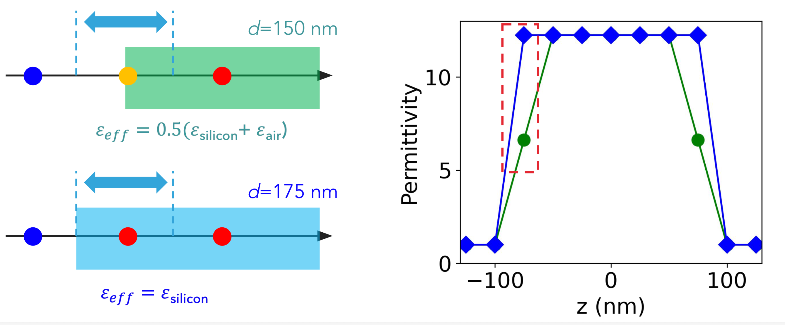
However, in this 1D case, this averaging is accurate because the dominant electric field is parallel to the dielectric grid points.
You can learn more about the subpixel averaging derivation from Maxwell’s equations in 1D in this lecture: Introduction to subpixel averaging.
2D & 3D Usage Caveats
In 2D, the subpixel averaging implementation depends on the polarization (\(s\) or \(p\)) of the incident electric field on the interface.
In 3D, the subpixel averaging is implemented with tensorial averaging due to arbitrary surface and field spatial orientations.
See also
- store_port_modes#
- port_offsets#
- sweep_spec#
- constraint#
- plot_eme_ports(x=None, y=None, z=None, ax=None, hlim=None, vlim=None, **kwargs)[source]#
Plot the EME ports.
- plot_eme_subgrid_boundaries(eme_grid_spec, x=None, y=None, z=None, ax=None, hlim=None, vlim=None, **kwargs)[source]#
Plot the EME subgrid boundaries. Does nothing if
eme_grid_specis notEMECompositeGrid. Operates recursively on subgrids.
- plot_eme_grid(x=None, y=None, z=None, ax=None, hlim=None, vlim=None, **kwargs)[source]#
Plot the EME grid.
- plot(x=None, y=None, z=None, ax=None, source_alpha=None, monitor_alpha=None, hlim=None, vlim=None, **patch_kwargs)[source]#
Plot each of simulation’s components on a plane defined by one nonzero x,y,z coordinate.
- Parameters:
x (float = None) – position of plane in x direction, only one of x, y, z must be specified to define plane.
y (float = None) – position of plane in y direction, only one of x, y, z must be specified to define plane.
z (float = None) – position of plane in z direction, only one of x, y, z must be specified to define plane.
source_alpha (float = None) – Opacity of the sources. If
None, uses Tidy3d default.monitor_alpha (float = None) – Opacity of the monitors. If
None, uses Tidy3d default.ax (matplotlib.axes._subplots.Axes = None) – Matplotlib axes to plot on, if not specified, one is created.
hlim (Tuple[float, float] = None) – The x range if plotting on xy or xz planes, y range if plotting on yz plane.
vlim (Tuple[float, float] = None) – The z range if plotting on xz or yz planes, y plane if plotting on xy plane.
- Returns:
The supplied or created matplotlib axes.
- Return type:
matplotlib.axes._subplots.Axes
- property eme_grid#
The EME grid as defined by ‘eme_grid_spec’. An EME grid is a 1D grid aligned with the propagation axis, dividing the simulation into cells. Modes and mode coefficients are defined at the central plane of each cell. Typically, cell boundaries are aligned with interfaces between structures in the simulation.
This is distinct from ‘grid’, which is the grid used in the tangential directions as well as the grid used for field monitors.
- classmethod from_scene(scene, **kwargs)[source]#
Create an EME simulation from a :class:.`Scene` instance. Must provide additional parameters to define a valid EME simulation (for example,
size,grid_spec, etc).- Parameters:
scene (:class:.`Scene`) – Scene containing structures information.
**kwargs – Other arguments
- property mode_solver_monitors#
A list of mode solver monitors at the cell centers. Each monitor has a mode spec. The cells and mode specs are specified by ‘eme_grid_spec’.
- property port_modes_monitor#
EME Mode solver monitor for only the port modes.
- property monitors_data_size#
Dictionary mapping monitor names to their estimated storage size in bytes.
- property max_num_modes#
Max number of modes in the simulation.
- property max_port_modes#
Max number of modes at the two ports.
- property grid#
Grid spatial locations and information as defined by grid_spec. This is the grid used in the tangential directions as well as the grid used for field monitors. This is distinct from ‘eme_grid’, which is the grid used for mode solving and EME propagation.
- __hash__()#
Hash method.