Self-intersecting PolySlab

This tutorial shows how to use the ComplexPolySlab plugin in tidy3d to deal with self-intersecting polygon that occurs during extrusion in a slanted polyslab.

import numpy as np
import matplotlib.pyplot as plt
import gdstk

import tidy3d as td

from tidy3d.plugins.polyslab import ComplexPolySlab

Example 1: concave polygon on the top with positive sidewall angle

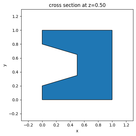
Let’s consider a concave polygon as shown in the following figure. As we dilate the polygon, the length of the edge in the middle will approach 0, and the two vertices at the end of the edge can be degenerate. Further dilation will result in a self-intersecting polygon. The collapsing of the two neighboring vertices is known as one type of edge events. There are other types of edge events as well, while our plugin at the moment will focus on this type of edge event.

vertices = (
    (0, 0),
    (1, 0),
    (1, 1),
    (0, 1),
    (0, 0.8),
    (0.5, 0.65),
    (0.5, 0.35),
    (0, 0.2),
)
s = td.PolySlab(
    vertices=vertices,
    slab_bounds=(0, 1),
    axis=2,
    sidewall_angle=0,
    reference_plane="top",
)
s.plot(z=0.5)
plt.show()

For a slanted polyslab where this polygon is at the top, self-intersection can occur as the polygon is extruded to the base when the sidewall angle is large. Since td.PolySlab only deals with simple polyslab, an error message will be displayed in this case.

sidewall_angle = np.pi / 4
try:
    s = td.PolySlab(
        vertices=vertices,
        slab_bounds=(0, 1),
        axis=2,
        sidewall_angle=sidewall_angle,
        reference_plane="top",
    )
except Exception as e:
    pass

[15:54:37] ERROR: Sidewall angle or structure thickness is so large that the        log.py:50
           polygon is self-intersecting during extrusion. Please either reduce               
           structure thickness to be < 2.016e-01, or use our plugin                          
           'ComplexPolySlab' to divide the complex polyslab into a list of simple            
           polyslabs.                                                                        

Dividing a complex polyslab into sub-polyslabs

The plugin ComplexPolySlab can divide such a complex polyslab into a list of simple polyslabs. The procedure of setting up the object is the same as in td.PolySlab:

s = ComplexPolySlab(
    vertices=vertices,
    slab_bounds=(0, 1),
    axis=2,
    sidewall_angle=sidewall_angle,
    reference_plane="top",
)

We can obtain the division result in the form of a list of simple polyslabs, or combined into a GeometryGroup. As shown below, the entire polyslab will be divided into 3 simple polyslabsl

# To obtain the divided polyslabs, there are two approaches:
# 1) a list of divided polyslabs
sub_polyslabs = s.sub_polyslabs

# 2) geometry group containing the divided polyslabs
polyslabs_group = s.geometry_group

print(f"The number of sub-polyslabs in the list is {len(sub_polyslabs)}.")
print(
    f"The number of sub-polyslabs in geometry group is {len(polyslabs_group.geometries)}."
)

The number of sub-polyslabs in the list is 3.
The number of sub-polyslabs in geometry group is 3.

Define a simulation

Now let’s make a simple simulation with a ComplexPolySlab object.

mat = td.Medium(permittivity=2)

# Three equivalent approaches
# 1) from sub-polyslabs
struct_list = [td.Structure(geometry=poly, medium=mat) for poly in s.sub_polyslabs]

# 2) from geometry group
struct_list = [td.Structure(geometry=s.geometry_group, medium=mat)]

# 3) directly obtain the structure with a user-specified medium
struct_list = [s.to_structure(mat)]

sim = td.Simulation(
    run_time=1e-12,
    size=(4, 4, 2),
    center=(0.5, 0.5, 0.5),
    grid_spec=td.GridSpec.auto(wavelength=1.0),
    structures=struct_list,
)

[15:54:38] WARNING: No sources in simulation.                                       log.py:50

Note: Tidy3D is warning us that our Simulation does not contain sources. In this case, since we are using the simulation as a demonstration and are not running any simulations, we may safely ignore this warning throughout this notebook.

Visualization

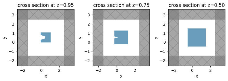
Three characteristic normal cross sections are illustrated below. The polygon near the top looks similar to the supplied polygon. Somewhere between \(z=0.75\) \(\mu\)m and \(z=0.95\) \(\mu\)m, a vertex-vertex crossing event happens, and the shape of the polygon changes. Between \(z=0.75\) \(\mu\)m and \(z=0.5\) \(\mu\)m, another event occurs, and the shape evolves to a simple box.

fig, ax = plt.subplots(1, 3, figsize=(8, 4), layout="tight")
sim.plot(z=0.95, ax=ax[0])
sim.plot(z=0.75, ax=ax[1])
sim.plot(z=0.5, ax=ax[2])
plt.show()

Example 2: GDS import

Similar to PolySlab, a ComplexPolySlab can also be setup from a gdstk.Cell. To illustrate this, let’s make a GDS cell with the aforementioned concave polygon, and load it with .from_gds classmethod.

# add the concave polygon to the gds cell

lib = gdstk.Library()
cell = lib.new_cell("SI")
poly = gdstk.Polygon(vertices, layer=0)
_ = cell.add(poly)

Loading a GDS cell into ComplexPolySlab

# obtain a list of polyslabs
geo_list = ComplexPolySlab.from_gds(
    cell,
    gds_layer=0,
    axis=2,
    slab_bounds=(0, 1),
    sidewall_angle=np.pi / 4,
    reference_plane="top",
)

structure = td.Structure(
    geometry=td.GeometryGroup(geometries=geo_list),
    medium=mat,
)

sim = td.Simulation(
    run_time=1e-12,
    size=(4, 4, 2),
    center=(0.5, 0.5, 0.5),
    grid_spec=td.GridSpec.auto(wavelength=1.0),
    structures=[structure],
)

           WARNING: No sources in simulation.                                       log.py:50

fig, ax = plt.subplots(1, 3, figsize=(8, 4), layout="tight")
sim.plot(z=0.95, ax=ax[0])
sim.plot(z=0.75, ax=ax[1])
sim.plot(z=0.5, ax=ax[2])
plt.show()