Boundary conditions
Contents
Boundary conditions#
Run this notebook in your browser using Binder.
This notebook will give a tutorial on setting up boundary conditions in Tidy3d.
[1]:
# standard python imports
import numpy as np
import matplotlib.pyplot as plt

# tidy3d imports
import tidy3d as td
import tidy3d.web as web
[12:04:30] INFO Using client version: 1.8.0 __init__.py:112
Define Simulation Parameters#
First, we’ll define some basc simulation parameters, the size of the domain, and the discretization resolution.
[2]:
# Define material properties
medium = td.Medium(permittivity=2)

wavelength = 1
f0 = td.C_0 / wavelength / np.sqrt(medium.permittivity)

# Set the domain size in x, y, and z
domain_size = 12 * wavelength

# create the geometry
geometry = []

# construct simulation size array
sim_size = (domain_size, domain_size, domain_size)

# Bandwidth in Hz
fwidth = f0 / 40.0

# Gaussian source offset; the source peak is at time t = offset/fwidth
offset = 4.0

# time dependence of sources
source_time = td.GaussianPulse(freq0=f0, fwidth=fwidth, offset=offset)

# Simulation run time past the source decay (around t=2*offset/fwidth)
run_time = 40 / fwidth
Create sources and monitors#
To study the effect of the various boundary conditions, we’ll define a point dipole source and a series of frequency- and time-domain monitors in the volume of the simulation domain and at its edges.
[3]:
# create a point dipole source
dipole = td.PointDipole(
    center=(0, 0, 0),
    source_time=source_time,
    polarization="Ex",
)

# these monitors will be used to plot fields on planes through the middle of the domain in the frequency domain
monitor_xz_freq = td.FieldMonitor(
    center=(0, 0, 0), size=(domain_size, 0, domain_size), freqs=[f0], name="xz_freq"
)
monitor_yz_freq = td.FieldMonitor(
    center=(0, 0, 0), size=(0, domain_size, domain_size), freqs=[f0], name="yz_freq"
)
monitor_xy_freq = td.FieldMonitor(
    center=(0, 0, 0), size=(domain_size, domain_size, 0), freqs=[f0], name="xy_freq"
)

# this monitor will be used to plot fields on a plane through the middle of the domain in the time domain
monitor_xz_time = td.FieldTimeMonitor(
    center=(0, 0, 0), size=(domain_size, 0, domain_size), interval=50, name="xz_time"
)
Boundary specifications#
A `BoundarySpec <https://docs.flexcompute.com/projects/tidy3d/en/latest/_autosummary/tidy3d.BoundarySpec.html>`__ object defines the boundary conditions applied on each of the 6 domain edges, and is provided as an input to the simulation. In the following sections, we’ll explore several different features within `BoundarySpec <https://docs.flexcompute.com/projects/tidy3d/en/latest/_autosummary/tidy3d.BoundarySpec.html>`__ and different ways of defining it.
A `BoundarySpec <https://docs.flexcompute.com/projects/tidy3d/en/latest/_autosummary/tidy3d.BoundarySpec.html>`__ consists of three `Boundary <https://docs.flexcompute.com/projects/tidy3d/en/latest/_autosummary/tidy3d.Boundary.html>`__ objects, each defining the boundaries on the plus and minus side of each dimension. A number of convenience functions are available to quickly define various types of boundaries, which will be demonstrated below.
Example 1: Default PML boundaries along some dimensions#
In most cases, one just wants to specify whether there are absorbing PML layers along any of the x, y, z dimensions. To do this, we can call the BoundarySpec.pml(x=False, y=False, z=False) method to construct boundary conditions, supplying True along a dimension where we want PML.
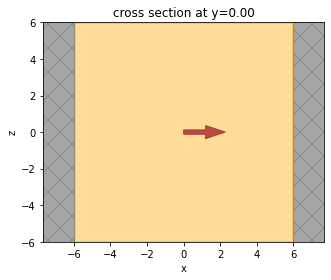
Let’s try putting pml on only the x edge.
[4]:
# define a basic boundary spec setting PML in along x only
bspec_pml = td.BoundarySpec.pml(x=True)

sim = td.Simulation(
    size=sim_size,
    sources=[dipole],
    monitors=[monitor_xz_time],
    run_time=run_time,
    boundary_spec=bspec_pml,
)

ax = sim.plot(y=0)
           INFO     Auto meshing using wavelength 1.4142 defined from        grid_spec.py:510
                    sources.
<Figure size 432x288 with 1 Axes>
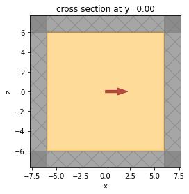
Now, let’s test by placing PMLs along all edges using the convenience method all_sides() and running the simulation.
[5]:
# define a basic boundary spec setting PML in all directions
bspec_pml = td.BoundarySpec.all_sides(boundary=td.PML())

# initialize the simulation object with the above boundary spec and source
sim = td.Simulation(
    size=sim_size,
    sources=[dipole],
    monitors=[monitor_xz_time],
    run_time=run_time,
    boundary_spec=bspec_pml,
)

# Visualize the geometry
fig, ax1 = plt.subplots(figsize=(4, 4))
sim.plot(y=0, ax=ax1)
           INFO     Auto meshing using wavelength 1.4142 defined from        grid_spec.py:510
                    sources.
<AxesSubplot: title={'center': 'cross section at y=0.00'}, xlabel='x', ylabel='z'>
<Figure size 288x288 with 1 Axes>
[6]:
sim_data = web.run(sim, task_name="bc_example1", path="data/bc_example1.hdf5")
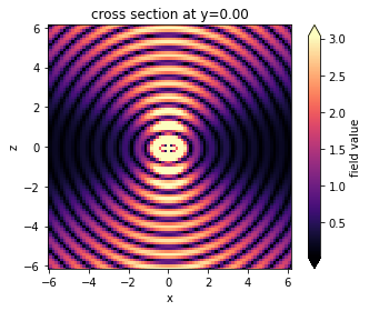
Visualize results#
We can observe the effect of the PML by looking at the fields in the time domain as they impinge on the boundaries. The figure shows that the fields are absorbed by the PML layers as expected, and no reflections are observed.
[7]:
fig, ax = plt.subplots(tight_layout=True, figsize=(5, 4))
sim_data.plot_field(
    field_monitor_name="xz_time", field_name="Ex", y=0, val="abs", t=2e-13, ax=ax
)

plt.show()
           INFO     Auto meshing using wavelength 1.4142 defined from        grid_spec.py:510
                    sources.
<Figure size 360x288 with 2 Axes>
Example 2: different boundaries on different edges#
Here, we’ll place a PML along the y and z directions. In the x direction, we’ll place a PML on the left side (x-minus), and a PEC on the right (x-plus). To specify individual boundary conditions along different dimensions, instead of `BoundarySpec <https://docs.flexcompute.com/projects/tidy3d/en/latest/_autosummary/tidy3d.BoundarySpec.html>`__, the class `Boundary <https://docs.flexcompute.com/projects/tidy3d/en/latest/_autosummary/tidy3d.Boundary.html>`__ is used, which defines the plus
and minus boundaries along a single dimension.
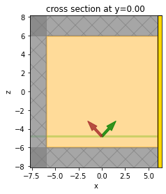
We’ll test this set of boundaries by placing an angled Gaussian beam near the lower edge of the domain and observing the field bounce off the PEC in x-plus.
[8]:
# this defines a 1D boundary with a PML on both the plus and minus sides, which can be reused for both y and z directions
boundary_yz = td.Boundary.pml(num_layers=15)

# this defines a 1D boundary with a PML on the minus side and a PEC on the plus side
boundary_x = td.Boundary(minus=td.PML(), plus=td.PECBoundary())

# now just set these in the boundary spec along the appropriate dimensions
bspec_pml_pec = td.BoundarySpec(x=boundary_x, y=boundary_yz, z=boundary_yz)


# create the Gaussian beam source
buffer_source = (
    domain_size / 10
)  # distance between the source and the bottom of the domain
gaussian_beam = td.GaussianBeam(
    center=(0, 0, -domain_size / 2 + buffer_source),
    size=(td.inf, td.inf, 0),
    source_time=source_time,
    direction="+",
    pol_angle=0,
    angle_theta=np.pi / 4.0,
    angle_phi=np.pi / 8.0,
    waist_radius=wavelength * 2,
    waist_distance=-wavelength * 4,
)

# initialize the simulation object with the above boundary spec and source
sim = td.Simulation(
    size=sim_size,
    sources=[gaussian_beam],
    monitors=[monitor_xz_time],
    run_time=run_time,
    boundary_spec=bspec_pml_pec,
)
We can verify that the PML is placed only on the left hand side and not on the right.
[9]:
# Visualize the geometry
fig, ax1 = plt.subplots(figsize=(4, 4))
sim.plot(y=0, ax=ax1)
[12:04:55] INFO     Auto meshing using wavelength 1.4142 defined from        grid_spec.py:510
                    sources.
<AxesSubplot: title={'center': 'cross section at y=0.00'}, xlabel='x', ylabel='z'>
<Figure size 288x288 with 1 Axes>
Run Simulation#
[10]:
sim_data = web.run(sim, task_name="bc_example2", path="data/bc_example2.hdf5")
Visualize results#
We can observe the effect of the PEC on x-plus by looking at the fields in the time domain as they bounce off the PEC boundary, as shown in the figure. Furthermore, the z-component of the electric field, which is tangential to the PEC boundary, goes to 0 at the boundary as expected.
[11]:
fig, (ax1, ax2) = plt.subplots(1, 2, tight_layout=True, figsize=(10, 4))
sim_data.plot_field(
    field_monitor_name="xz_time", field_name="Ex", y=0, val="abs", t=2e-13, ax=ax1
)
sim_data.plot_field(
    field_monitor_name="xz_time", field_name="Ez", y=0, val="abs", t=2e-13, ax=ax2
)
plt.show()
[12:05:17] INFO     Auto meshing using wavelength 1.4142 defined from        grid_spec.py:510
                    sources.
<Figure size 720x288 with 4 Axes>
Example 3: different boundaries on different edges#
Next, let’s consider an even more general setup where all 6 boundaries of the domain are individually specified, and different types of boundaries are mixed in the plus and minus sides along each dimension.
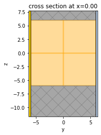
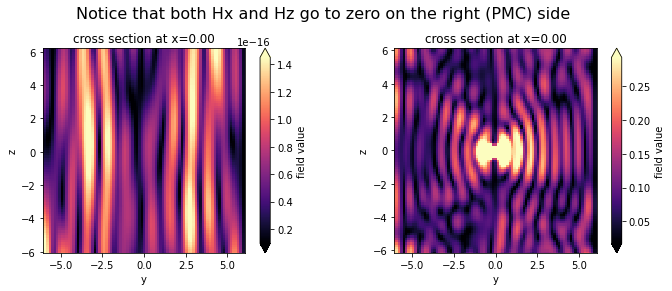
We’ll test this set of boundaries by placing the point dipole at the center of the domain again, this time studying the fields at the edges of the domain and checking that the various tangential field components satisfy the PEC and PMC boundary conditions as expected from theory.
[12]:
# define the boundary spec
bspec_general = td.BoundarySpec(
    x=td.Boundary(minus=td.Periodic(), plus=td.PECBoundary()),
    y=td.Boundary(minus=td.PECBoundary(), plus=td.PMCBoundary()),
    z=td.Boundary(minus=td.Absorber(), plus=td.PML()),
)
# note that when a periodic boundary is applied across from a PEC (PMC), the periodic boundary is just replaced by the PEC (PMC).


# initialize the simulation object with the above boundary spec and the dipole source from earlier
sim = td.Simulation(
    size=sim_size,
    sources=[dipole],
    monitors=[monitor_xz_freq, monitor_yz_freq, monitor_xy_freq],
    run_time=run_time,
    boundary_spec=bspec_general,
)

# Visualize the geometry
fig, ax1 = plt.subplots(figsize=(4, 4))
sim.plot(x=0, ax=ax1)
           WARNING  A periodic boundary condition was specified on the        boundary.py:399
                    opposide side of a perfect electric or magnetic conductor
                    boundary. This periodic boundary condition will be
                    replaced by the perfect electric or magnetic conductor
                    across from it.
           INFO     Auto meshing using wavelength 1.4142 defined from        grid_spec.py:510
                    sources.
<AxesSubplot: title={'center': 'cross section at x=0.00'}, xlabel='y', ylabel='z'>
<Figure size 288x288 with 1 Axes>
Run Simulation#
[13]:
sim_data = web.run(sim, task_name="bc_example3", path="data/bc_example3.hdf5")
Visualize results#
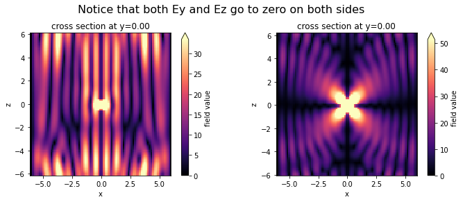
In x-plus, we have a PEC, so Ey and Ez should be nearly zero on the x-plus boundary.
In x-minus we have a periodic condition across from the PEC in x-plus, which just means that there’s also a PEC in x-minus. So again Ey and Ez should be nearly zero on the x-minus boundary.
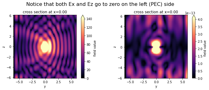
In y-minus, we have another PEC, so Ex and Ez should be nearly zero on the y-minus boundary.
In y-plus, we have a PMC, so Hx and Hz should be nearly zero on the y-plus boundary.
Each of these cases is verified below.
[14]:
fig, (ax1, ax2) = plt.subplots(1, 2, tight_layout=True, figsize=(10, 4))
sim_data.plot_field(
    field_monitor_name="xz_freq", field_name="Ey", y=0, val="abs", freq=f0, ax=ax1
)
sim_data.plot_field(
    field_monitor_name="xz_freq", field_name="Ez", y=0, val="abs", freq=f0, ax=ax2
)
fig.suptitle("Notice that both Ey and Ez go to zero on both sides", fontsize=16)

fig, (ax1, ax2) = plt.subplots(1, 2, tight_layout=True, figsize=(10, 4))
sim_data.plot_field(
    field_monitor_name="yz_freq", field_name="Ex", x=0, val="abs", freq=f0, ax=ax1
)
sim_data.plot_field(
    field_monitor_name="yz_freq", field_name="Ez", x=0, val="abs", freq=f0, ax=ax2
)
fig.suptitle(
    "Notice that both Ex and Ez go to zero on the left (PEC) side", fontsize=16
)

fig, (ax1, ax2) = plt.subplots(1, 2, tight_layout=True, figsize=(10, 4))
sim_data.plot_field(
    field_monitor_name="yz_freq", field_name="Hx", x=0, val="abs", freq=f0, ax=ax1
)
sim_data.plot_field(
    field_monitor_name="yz_freq", field_name="Hz", x=0, val="abs", freq=f0, ax=ax2
)
fig.suptitle(
    "Notice that both Hx and Hz go to zero on the right (PMC) side", fontsize=16
)
plt.show()
           WARNING  'freq' suppled to 'plot_field', frequency selection key   sim_data.py:325
                    renamed to 'f' and 'freq' will error in future release,
                    please update your local script to use 'f=value'.
           INFO     Auto meshing using wavelength 1.4142 defined from        grid_spec.py:510
                    sources.
           WARNING  'freq' suppled to 'plot_field', frequency selection key   sim_data.py:325
                    renamed to 'f' and 'freq' will error in future release,
                    please update your local script to use 'f=value'.
           WARNING  'freq' suppled to 'plot_field', frequency selection key   sim_data.py:325
                    renamed to 'f' and 'freq' will error in future release,
                    please update your local script to use 'f=value'.
[12:06:01] WARNING  'freq' suppled to 'plot_field', frequency selection key   sim_data.py:325
                    renamed to 'f' and 'freq' will error in future release,
                    please update your local script to use 'f=value'.
           WARNING  'freq' suppled to 'plot_field', frequency selection key   sim_data.py:325
                    renamed to 'f' and 'freq' will error in future release,
                    please update your local script to use 'f=value'.
           WARNING  'freq' suppled to 'plot_field', frequency selection key   sim_data.py:325
                    renamed to 'f' and 'freq' will error in future release,
                    please update your local script to use 'f=value'.
<Figure size 720x288 with 4 Axes>
<Figure size 720x288 with 4 Axes>
<Figure size 720x288 with 4 Axes>
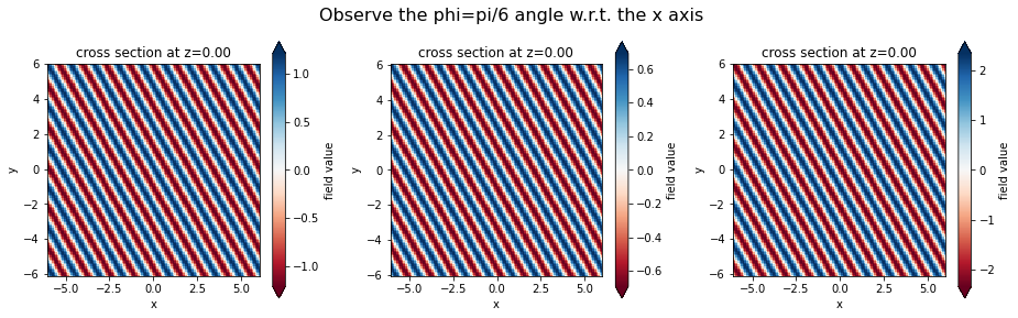
Example 4: Bloch boundary conditions along x and y to allow injecting an angled plane wave source#
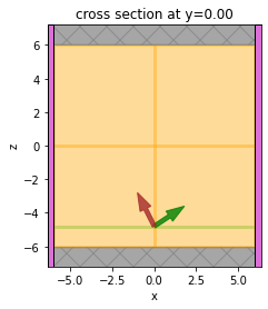
Finally, we’ll use the Bloch boundary condition in combination with a plane wave source to demonstrate the injection of an angled plane wave. The Bloch boundaries are used along the x and y dimensions, while PMLs are used along z. The Bloch vectors are automatically computed based on the angles defined in the plane wave source. A dielectric background medium with a relative permittivity of 2 is used.
We’ll test this set of boundaries by placing an angled plane wave near the lower edge of the domain and observing the plane wave in the frequency domain.
[15]:
# First, define the plane wave source, since it is needed to define the Bloch boundary in this case.
# Note that in general, the Bloch boundary can also be defined by just providing a bandstructure-normalized Bloch vector.

buffer_source = (
    domain_size / 10
)  # distance between the source and the bottom of the domain
plane_wave = td.PlaneWave(
    center=(0, 0, -domain_size / 2 + buffer_source),
    size=(td.inf, td.inf, 0),
    source_time=source_time,
    direction="+",
    pol_angle=0,
    angle_theta=np.pi / 3.0,
    angle_phi=np.pi / 6.0,
)


# create the Bloch boundaries
bloch_x = td.Boundary.bloch_from_source(
    source=plane_wave, domain_size=sim_size[0], axis=0, medium=medium
)
bloch_y = td.Boundary.bloch_from_source(
    source=plane_wave, domain_size=sim_size[1], axis=1, medium=medium
)

bspec_bloch = td.BoundarySpec(x=bloch_x, y=bloch_y, z=td.Boundary.pml())


# initialize the simulation object with the above boundary spec and source
sim = td.Simulation(
    size=sim_size,
    sources=[plane_wave],
    monitors=[monitor_xz_freq, monitor_yz_freq, monitor_xy_freq],
    run_time=run_time,
    boundary_spec=bspec_bloch,
    medium=medium,
)

# Visualize the geometry
fig, ax1 = plt.subplots(figsize=(4, 4))
sim.plot(y=0, ax=ax1)
[12:06:02] INFO     Auto meshing using wavelength 1.4142 defined from        grid_spec.py:510
                    sources.
<AxesSubplot: title={'center': 'cross section at y=0.00'}, xlabel='x', ylabel='z'>
<Figure size 288x288 with 1 Axes>
Run Simulation#
[16]:
sim_data = web.run(sim, task_name="bc_example4", path="data/bc_example4.hdf5")
Visualize results#
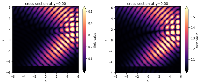
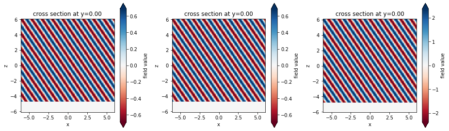
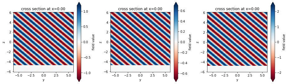
In shown in the plots, the plane wave is successfully injected at the specified angles without reflections.
[17]:
fig, (ax1, ax2, ax3) = plt.subplots(1, 3, tight_layout=True, figsize=(13, 4))
sim_data.plot_field(
    field_monitor_name="xz_freq", field_name="Ey", y=0, val="real", f=f0, ax=ax1
)
sim_data.plot_field(
    field_monitor_name="xz_freq", field_name="Ey", y=0, val="real", f=f0, ax=ax2
)
sim_data.plot_field(
    field_monitor_name="xz_freq", field_name="Ez", y=0, val="real", f=f0, ax=ax3
)

fig, (ax1, ax2, ax3) = plt.subplots(1, 3, tight_layout=True, figsize=(13, 4))
sim_data.plot_field(
    field_monitor_name="yz_freq", field_name="Ex", x=0, val="real", f=f0, ax=ax1
)
sim_data.plot_field(
    field_monitor_name="yz_freq", field_name="Ey", x=0, val="real", f=f0, ax=ax2
)
sim_data.plot_field(
    field_monitor_name="yz_freq", field_name="Ez", x=0, val="real", f=f0, ax=ax3
)

fig, (ax1, ax2, ax3) = plt.subplots(1, 3, tight_layout=True, figsize=(13, 4))
sim_data.plot_field(
    field_monitor_name="xy_freq", field_name="Ex", z=0, val="real", f=f0, ax=ax1
)
sim_data.plot_field(
    field_monitor_name="xy_freq", field_name="Ey", z=0, val="real", f=f0, ax=ax2
)
sim_data.plot_field(
    field_monitor_name="xy_freq", field_name="Ez", z=0, val="real", f=f0, ax=ax3
)
fig.suptitle("Observe the phi=pi/6 angle w.r.t. the x axis", fontsize=16)

plt.show()
           INFO     Auto meshing using wavelength 1.4142 defined from        grid_spec.py:510
                    sources.
<Figure size 936x288 with 6 Axes>
<Figure size 936x288 with 6 Axes>
<Figure size 936x288 with 6 Axes>
Summary#
The fastest way to define boundary conditions with periodic and absorbing boundaries on some sides is through
td.BoundarySpec.pml(y=True)(i.e., for PML along y only), or throughtd.BoundarySpec.all_sides(boundary=PML())to set the same boundary on all sides (in this example, PML on all sides).To further fine tune the global boundary specifications, use BoundarySpec(x, y, z), where x, y, z are Boundary objects.
Boundary objects have some convenience methods, like
.pml()for defining the boundaries along an edge with more parameters.Boundary objects can be further specified by supplying boundary conditions to the
plusandminusfields.
[ ]: