tidy3d.Simulation

class Simulation

Bases: AbstractYeeGridSimulation

Custom implementation of Maxwell’s equations which represents the physical model to be solved using the FDTD method.

Parameters:

• attrs (dict = {}) – Dictionary storing arbitrary metadata for a Tidy3D object. This dictionary can be freely used by the user for storing data without affecting the operation of Tidy3D as it is not used internally. Note that, unlike regular Tidy3D fields, attrs are mutable. For example, the following is allowed for setting an attr obj.attrs['foo'] = bar. Also note that Tidy3D` will raise a TypeError if attrs contain objects that can not be serialized. One can check if attrs are serializable by calling obj.json().

• center (Union[tuple[Union[float, autograd.tracer.Box], Union[float, autograd.tracer.Box], Union[float, autograd.tracer.Box]], Box] = (0.0, 0.0, 0.0)) – [units = um]. Center of object in x, y, and z.

• size (Union[tuple[Union[pydantic.v1.types.NonNegativeFloat, autograd.tracer.Box], Union[pydantic.v1.types.NonNegativeFloat, autograd.tracer.Box], Union[pydantic.v1.types.NonNegativeFloat, autograd.tracer.Box]], Box]) – [units = um]. Size in x, y, and z directions.

• medium (Union[Medium, AnisotropicMedium, PECMedium, PoleResidue, Sellmeier, Lorentz, Debye, Drude, FullyAnisotropicMedium, CustomMedium, CustomPoleResidue, CustomSellmeier, CustomLorentz, CustomDebye, CustomDrude, CustomAnisotropicMedium, PerturbationMedium, PerturbationPoleResidue, LossyMetalMedium] = Medium(attrs={}, name=None, frequency_range=None, allow_gain=False, nonlinear_spec=None, modulation_spec=None, viz_spec=None, heat_spec=None, type='Medium', permittivity=1.0, conductivity=0.0)) – Background medium of simulation, defaults to vacuum if not specified.

• structures (Tuple[Structure, ...] = ()) – Tuple of structures present in simulation. Note: Structures defined later in this list override the simulation material properties in regions of spatial overlap.

• symmetry (Tuple[Literal[0, -1, 1], Literal[0, -1, 1], Literal[0, -1, 1]] = (0, 0, 0)) – Tuple of integers defining reflection symmetry across a plane bisecting the simulation domain normal to the x-, y-, and z-axis at the simulation center of each axis, respectively. Each element can be 0 (no symmetry), 1 (even, i.e. ‘PMC’ symmetry) or -1 (odd, i.e. ‘PEC’ symmetry). Note that the vectorial nature of the fields must be taken into account to correctly determine the symmetry value.

• sources (Tuple[Annotated[Union[tidy3d.components.source.current.UniformCurrentSource, tidy3d.components.source.current.PointDipole, tidy3d.components.source.field.GaussianBeam, tidy3d.components.source.field.AstigmaticGaussianBeam, tidy3d.components.source.field.ModeSource, tidy3d.components.source.field.PlaneWave, tidy3d.components.source.field.CustomFieldSource, tidy3d.components.source.current.CustomCurrentSource, tidy3d.components.source.field.TFSF], FieldInfo(default=PydanticUndefined, discriminator='type', extra={})], ...] = ()) – Tuple of electric current sources injecting fields into the simulation.

• boundary_spec (BoundarySpec = BoundarySpec(attrs={}, x=Boundary(attrs={},, plus=PML(attrs={},, name=None,, type='PML',, num_layers=12,, parameters=PMLParams(attrs={},, sigma_order=3,, sigma_min=0.0,, sigma_max=1.5,, type='PMLParams',, kappa_order=3,, kappa_min=1.0,, kappa_max=3.0,, alpha_order=1,, alpha_min=0.0,, alpha_max=0.0)),, minus=PML(attrs={},, name=None,, type='PML',, num_layers=12,, parameters=PMLParams(attrs={},, sigma_order=3,, sigma_min=0.0,, sigma_max=1.5,, type='PMLParams',, kappa_order=3,, kappa_min=1.0,, kappa_max=3.0,, alpha_order=1,, alpha_min=0.0,, alpha_max=0.0)),, type='Boundary'), y=Boundary(attrs={},, plus=PML(attrs={},, name=None,, type='PML',, num_layers=12,, parameters=PMLParams(attrs={},, sigma_order=3,, sigma_min=0.0,, sigma_max=1.5,, type='PMLParams',, kappa_order=3,, kappa_min=1.0,, kappa_max=3.0,, alpha_order=1,, alpha_min=0.0,, alpha_max=0.0)),, minus=PML(attrs={},, name=None,, type='PML',, num_layers=12,, parameters=PMLParams(attrs={},, sigma_order=3,, sigma_min=0.0,, sigma_max=1.5,, type='PMLParams',, kappa_order=3,, kappa_min=1.0,, kappa_max=3.0,, alpha_order=1,, alpha_min=0.0,, alpha_max=0.0)),, type='Boundary'), z=Boundary(attrs={},, plus=PML(attrs={},, name=None,, type='PML',, num_layers=12,, parameters=PMLParams(attrs={},, sigma_order=3,, sigma_min=0.0,, sigma_max=1.5,, type='PMLParams',, kappa_order=3,, kappa_min=1.0,, kappa_max=3.0,, alpha_order=1,, alpha_min=0.0,, alpha_max=0.0)),, minus=PML(attrs={},, name=None,, type='PML',, num_layers=12,, parameters=PMLParams(attrs={},, sigma_order=3,, sigma_min=0.0,, sigma_max=1.5,, type='PMLParams',, kappa_order=3,, kappa_min=1.0,, kappa_max=3.0,, alpha_order=1,, alpha_min=0.0,, alpha_max=0.0)),, type='Boundary'), type='BoundarySpec')) – Specification of boundary conditions along each dimension. If None, PML boundary conditions are applied on all sides.

• monitors (Tuple[Annotated[Union[tidy3d.components.monitor.FieldMonitor, tidy3d.components.monitor.FieldTimeMonitor, tidy3d.components.monitor.PermittivityMonitor, tidy3d.components.monitor.FluxMonitor, tidy3d.components.monitor.FluxTimeMonitor, tidy3d.components.monitor.ModeMonitor, tidy3d.components.monitor.ModeSolverMonitor, tidy3d.components.monitor.FieldProjectionAngleMonitor, tidy3d.components.monitor.FieldProjectionCartesianMonitor, tidy3d.components.monitor.FieldProjectionKSpaceMonitor, tidy3d.components.monitor.DiffractionMonitor, tidy3d.components.monitor.DirectivityMonitor], FieldInfo(default=PydanticUndefined, discriminator='type', extra={})], ...] = ()) – Tuple of monitors in the simulation. Note: monitor names are used to access data after simulation is run.

• grid_spec (GridSpec = GridSpec(attrs={}, grid_x=AutoGrid(attrs={},, type='AutoGrid',, max_scale=1.4,, mesher=GradedMesher(attrs={},, type='GradedMesher'),, dl_min=None,, min_steps_per_wvl=10.0,, min_steps_per_sim_size=10.0), grid_y=AutoGrid(attrs={},, type='AutoGrid',, max_scale=1.4,, mesher=GradedMesher(attrs={},, type='GradedMesher'),, dl_min=None,, min_steps_per_wvl=10.0,, min_steps_per_sim_size=10.0), grid_z=AutoGrid(attrs={},, type='AutoGrid',, max_scale=1.4,, mesher=GradedMesher(attrs={},, type='GradedMesher'),, dl_min=None,, min_steps_per_wvl=10.0,, min_steps_per_sim_size=10.0), wavelength=None, override_structures=(), snapping_points=(), layer_refinement_specs=(), type='GridSpec')) – Specifications for the simulation grid along each of the three directions.

• version (str = 2.8.0rc3) – String specifying the front end version number.

• plot_length_units (Optional[Literal['nm', 'μm', 'um', 'mm', 'cm', 'm']] = μm) – When set to a supported LengthUnit, plots will be produced with proper scaling of axes and include the desired unit specifier in labels.

• lumped_elements (Tuple[Annotated[Union[tidy3d.components.lumped_element.LumpedResistor, tidy3d.components.lumped_element.CoaxialLumpedResistor, tidy3d.components.lumped_element.LinearLumpedElement], FieldInfo(default=PydanticUndefined, discriminator='type', extra={})], ...] = ()) – Tuple of lumped elements in the simulation.

• subpixel (Union[bool, SubpixelSpec] = SubpixelSpec(attrs={}, dielectric=PolarizedAveraging(attrs={},, type='PolarizedAveraging'), metal=Staircasing(attrs={},, type='Staircasing'), pec=PECConformal(attrs={},, type='PECConformal',, timestep_reduction=0.3), lossy_metal=SurfaceImpedance(attrs={},, type='SurfaceImpedance',, timestep_reduction=0.0), type='SubpixelSpec')) – Apply subpixel averaging methods of the permittivity on structure interfaces to result in much higher accuracy for a given grid size. Supply a SubpixelSpec to this field to select subpixel averaging methods separately on dielectric, metal, and PEC material interfaces. Alternatively, user may supply a boolean value: True to apply the default subpixel averaging methods corresponding to SubpixelSpec() , or False to apply staircasing.

• simulation_type (Optional[Literal['autograd_fwd', 'autograd_bwd', 'tidy3d', None]] = tidy3d) – Tag used internally to distinguish types of simulations for autograd gradient processing.

• post_norm (Union[float, FreqDataArray] = 1.0) – Factor to multiply the fields by after running, given the adjoint source pipeline used. Note: this is used internally only.

• courant (ConstrainedFloatValue = 0.99) – Normalized Courant stability factor that is no larger than 1 when CFL stability condition is met. It controls time step to spatial step ratio. Lower values lead to more stable simulations for dispersive materials, but result in longer simulation times.

• normalize_index (Optional[NonNegativeInt] = 0) – Index of the source in the tuple of sources whose spectrum will be used to normalize the frequency-dependent data. If None, the raw field data is returned unnormalized.

• shutoff (NonNegativeFloat = 1e-05) – Ratio of the instantaneous integrated E-field intensity to the maximum value at which the simulation will automatically terminate time stepping. Used to prevent extraneous run time of simulations with fully decayed fields. Set to 0 to disable this feature.

• run_time (Union[PositiveFloat, RunTimeSpec]) – [units = sec]. Total electromagnetic evolution time in seconds. Note: If simulation ‘shutoff’ is specified, simulation will terminate early when shutoff condition met. Alternatively, user may supply a RunTimeSpec to this field, which will auto-compute the run_time based on the contents of the spec. If this option is used, the evaluated run_time value is available in the Simulation._run_time property.

Notes

A Simulation defines a custom implementation of Maxwell’s equations which represents the physical model to be solved using the Finite-Difference Time-Domain (FDTD) method. tidy3d simulations run very quickly in the cloud through GPU parallelization.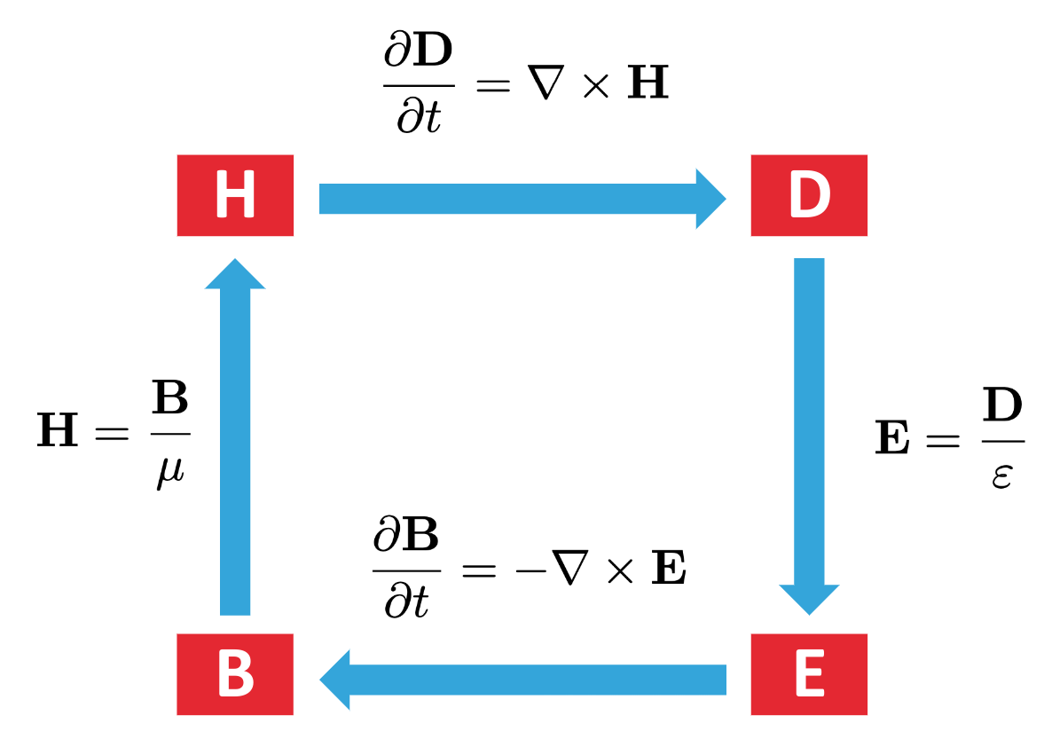

FDTD is a method for simulating the interaction of electromagnetic waves with structures and materials. It is the most widely used method in photonics design. The Maxwell’s equations implemented in the Simulation are solved per time-step in the order shown in this image.

The simplified input to FDTD solver consists of the permittivity distribution defined by structures which describe the device and sources of electromagnetic excitation. This information is used to computate the time dynamics of the electric and magnetic fields in this system. From these time-domain results, frequency-domain information of the simulation can also be extracted, and used for device design and optimization.

If you are new to the FDTD method, we recommend you get started with the FDTD 101 Lecture Series

Dimensions Selection

By default, simulations are defined as 3D. To make the simulation 2D, we can just set the simulation size in one of the dimensions to be 0. However, note that we still have to define a grid size (eg. tidy3d.Simulation(size=[size_x, size_y, 0])) and specify a periodic boundary condition in that direction.

See further parameter explanations below.

Example

>>> from tidy3d import Sphere, Cylinder, PolySlab
>>> from tidy3d import UniformCurrentSource, GaussianPulse
>>> from tidy3d import FieldMonitor, FluxMonitor
>>> from tidy3d import GridSpec, AutoGrid
>>> from tidy3d import BoundarySpec, Boundary
>>> from tidy3d import Medium
>>> sim = Simulation(
...     size=(3.0, 3.0, 3.0),
...     grid_spec=GridSpec(
...         grid_x = AutoGrid(min_steps_per_wvl = 20),
...         grid_y = AutoGrid(min_steps_per_wvl = 20),
...         grid_z = AutoGrid(min_steps_per_wvl = 20)
...     ),
...     run_time=40e-11,
...     structures=[
...         Structure(
...             geometry=Box(size=(1, 1, 1), center=(0, 0, 0)),
...             medium=Medium(permittivity=2.0),
...         ),
...     ],
...     sources=[
...         UniformCurrentSource(
...             size=(0, 0, 0),
...             center=(0, 0.5, 0),
...             polarization="Hx",
...             source_time=GaussianPulse(
...                 freq0=2e14,
...                 fwidth=4e13,
...             ),
...         )
...     ],
...     monitors=[
...         FluxMonitor(size=(1, 1, 0), center=(0, 0, 0), freqs=[2e14, 2.5e14], name='flux'),
...     ],
...     symmetry=(0, 0, 0),
...     boundary_spec=BoundarySpec(
...         x = Boundary.pml(num_layers=20),
...         y = Boundary.pml(num_layers=30),
...         z = Boundary.periodic(),
...     ),
...     shutoff=1e-6,
...     courant=0.8,
...     subpixel=False,
... )

See also

Notebooks:

• Quickstart: Usage in a basic simulation flow.

• Using automatic nonuniform meshing

• See nearly all notebooks for Simulation applications.

Lectures:

• Introduction to FDTD Simulation: Usage in a basic simulation flow.

• Prelude to Integrated Photonics Simulation: Mode Injection

GUI:

• FDTD Walkthrough

Attributes

all_structures	List of all structures in the simulation (including the Simulation.medium).
allow_gain	True if any of the mediums in the simulation allows gain.
background_structure	Returns structure representing the background of the Simulation.
complex_fields	Whether complex fields are used in the simulation.
custom_datasets	List of custom datasets for verification purposes.
dt	Simulation time step (distance).
freqs_adjoint	Unique list of all frequencies.
frequency_range	Range of frequencies spanning all sources' frequency dependence.
medium_map	Returns dict mapping medium to index in material.
mediums	Returns set of distinct AbstractMedium in simulation.
monitors_data_size	Dictionary mapping monitor names to their estimated storage size in bytes.
n_max	Maximum refractive index in the Simulation.
num_cells	Number of cells in the simulation grid.
num_computational_grid_points	Number of cells in the computational domain for this simulation.
num_time_steps	Number of time steps in simulation.
nyquist_step	Maximum number of discrete time steps to keep sampling below Nyquist limit.
scaled_courant	When conformal mesh is applied, courant number is scaled down depending on conformal_mesh_spec.
self_structure	The simulation background as a Structure.
tmesh	FDTD time stepping points.
wvl_mat_min	Minimum wavelength in the materials present throughout the simulation.
version	DO NOT EDIT: Modified automatically with .bump2version.cfg
attrs

Methods

bloch_boundaries_diff_mnt(val, values)	Error if there are diffraction monitors incompatible with boundary conditions.
bloch_with_symmetry(val, values)	Error if a Bloch boundary is applied with symmetry
boundaries_for_zero_dims(val, values)	Error if absorbing boundaries, bloch boundaries, unmatching pec/pmc, or symmetry is used along a zero dimension.
check_fixed_angle_components(values)	Error if a fixed-angle plane wave is combined with other sources or fully anisotropic mediums or gain mediums.
diffraction_monitor_boundaries(val, values)	If any DiffractionMonitor exists, ensure boundary conditions in the transverse directions are periodic or Bloch.
diffraction_monitor_medium(val, values)	If any DiffractionMonitor exists, ensure is does not lie in a lossy medium.
from_scene(scene, **kwargs)	Create a simulation from a Scene instance.
get_refractive_indices(freq)	List of refractive indices in the simulation at a given frequency.
intersecting_media(test_object, structures)	From a given list of structures, returns a list of AbstractMedium associated with those structures that intersect with the test_object, if it is a surface, or its surfaces, if it is a volume.
intersecting_structures(test_object, structures)	From a given list of structures, returns a list of Structure that intersect with the test_object, if it is a surface, or its surfaces, if it is a volume.
make_adjoint_monitors(sim_fields_keys)	Get lists of field and permittivity monitors for this simulation.
monitor_medium(monitor)	Return the medium in which the given monitor resides.
perturbed_mediums_copy([temperature, ...])	Return a copy of the simulation with heat and/or charge data applied to all mediums that have perturbation models specified.
plane_wave_boundaries(val, values)	Error if there are plane wave sources incompatible with boundary conditions.
plot_3d([width, height])	Render 3D plot of Simulation (in jupyter notebook only).
proj_distance_for_approx(val, values)	Warn if projection distance for projection monitors is not large compared to monitor or, simulation size, yet far_field_approx is True.
tfsf_boundaries(val, values)	Error if the boundary conditions are compatible with TFSF sources, if any.
tfsf_with_symmetry(val, values)	Error if a TFSF source is applied with symmetry
to_gds(cell[, x, y, z, ...])	Append the simulation structures to a .gds cell.
to_gds_file(fname[, x, y, z, ...])	Append the simulation structures to a .gds cell.
to_gdspy([x, y, z, gds_layer_dtype_map])	Convert a simulation's planar slice to a .gds type polygon list.
to_gdstk([x, y, z, permittivity_threshold, ...])	Convert a simulation's planar slice to a .gds type polygon list.
validate_pre_upload([source_required])	Validate the fully initialized simulation is ok for upload to our servers.
with_adjoint_monitors(sim_fields_keys)	Copy of self with adjoint field and permittivity monitors for every traced structure.

Inherited Common Usage

boundary_spec

Specification of boundary conditions along each dimension. If None, PML boundary conditions are applied on all sides.

Example

Simple application reference:

Simulation(
   ...
    boundary_spec=BoundarySpec(
       x = Boundary.pml(num_layers=20),
       y = Boundary.pml(num_layers=30),
       z = Boundary.periodic(),
   ),
   ...
)

See also

PML:

A perfectly matched layer model.

BoundarySpec:

Specifies boundary conditions on each side of the domain and along each dimension.

Index

All boundary condition models.

Notebooks

• How to troubleshoot a diverged FDTD simulation

Lectures

• Using FDTD to Compute a Transmission Spectrum

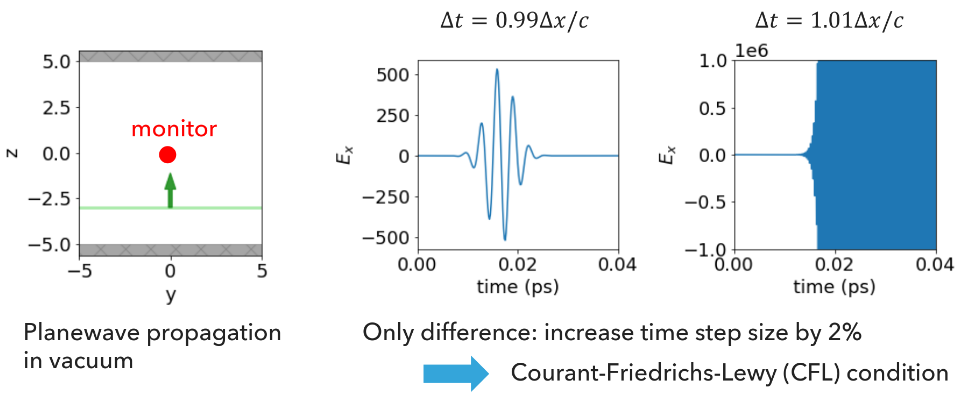
courant

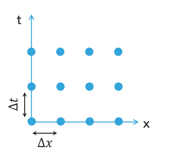
The Courant-Friedrichs-Lewy (CFL) stability factor \(C\), controls time step to spatial step ratio. A physical wave has to propagate slower than the numerical information propagation in a Yee-cell grid. This is because in this spatially-discrete grid, information propagates over 1 spatial step \(\Delta x\) over a time step \(\Delta t\). This constraint enables the correct physics to be captured by the simulation.

1D Illustration

In a 1D model:

Lower values lead to more stable simulations for dispersive materials, but result in longer simulation times. This factor is normalized to no larger than 1 when CFL stability condition is met in 3D.

For a 1D grid:

\[C_{\text{1D}} = \frac{c \Delta t}{\Delta x} \leq 1\]

2D Illustration

In a 2D uniform grid, where the \(E_z\) field is at the red dot center surrounded by four green magnetic edge components in a square Yee cell grid:

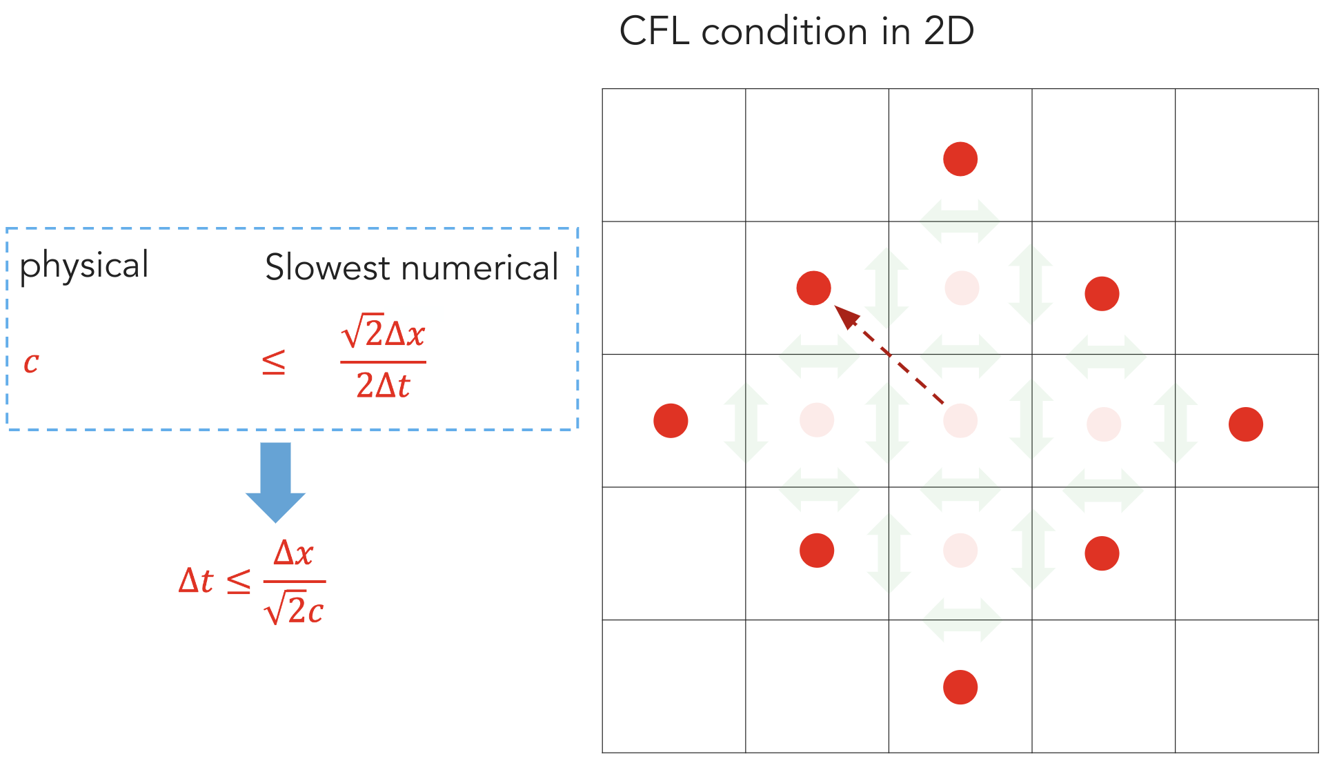\[C_{\text{2D}} = \frac{c\Delta t}{\Delta x} \leq \frac{1}{\sqrt{2}}\]

Hence, for the same spatial grid, the time step in 2D grid needs to be smaller than the time step in a 1D grid. Note we use a normalized Courant number in our simulation, which in 2D is \(\sqrt{2}C_{\text{2D}}\). CFL stability condition is met when the normalized Courant number is no larger than 1.

3D Illustration

For an isotropic medium with refractive index \(n\), the 3D time step condition can be derived to be:

\[\Delta t \le \frac{n}{c \sqrt{\frac{1}{\Delta x^2} + \frac{1}{\Delta y^2} + \frac{1}{\Delta z^2}}}\]

In this case, the number of spatial grid points scale by \(\sim \frac{1}{\Delta x^3}\) where \(\Delta x\) is the spatial discretization in the \(x\) dimension. If the total simulation time is kept the same whilst maintaining the CFL condition, then the number of time steps required scale by \(\sim \frac{1}{\Delta x}\). Hence, the spatial grid discretization influences the total time-steps required. The total simulation scaling per spatial grid size in this case is by \(\sim \frac{1}{\Delta x^4}.\)

As an example, in this case, refining the mesh by a factor or 2 (reducing the spatial step size by half) \(\Delta x \to \frac{\Delta x}{2}\) will increase the total simulation computational cost by 16.

Divergence Caveats

tidy3d uses a default Courant factor of 0.99. When a dispersive material with eps_inf < 1 is used, the Courant factor will be automatically adjusted to be smaller than sqrt(eps_inf) to ensure stability. If your simulation still diverges despite addressing any other issues discussed above, reducing the Courant factor may help.

See also

grid_spec

Specifications for the simulation grid along each of the three directions.

Lectures:

• Time step size and CFL condition in FDTD

• Numerical dispersion in FDTD

lumped_elements

Tuple of lumped elements in the simulation.

Example

Simple application reference:

Simulation(
   ...
   lumped_elements=[
       LumpedResistor(
           size=(0, 3, 1),
           center=(0, 0, 0),
           voltage_axis=2,
           resistance=50,
           name="resistor_1",
       )
   ],
   ...
)

See also

Lumped Elements:

Available lumped element types.

Notebooks:

• Using lumped elements in Tidy3D simulations

grid_spec

Specifications for the simulation grid along each of the three directions.

Example

Simple application reference:

Simulation(
   ...
    grid_spec=GridSpec(
       grid_x = AutoGrid(min_steps_per_wvl = 20),
       grid_y = AutoGrid(min_steps_per_wvl = 20),
       grid_z = AutoGrid(min_steps_per_wvl = 20)
   ),
   ...
)

Usage Recommendations

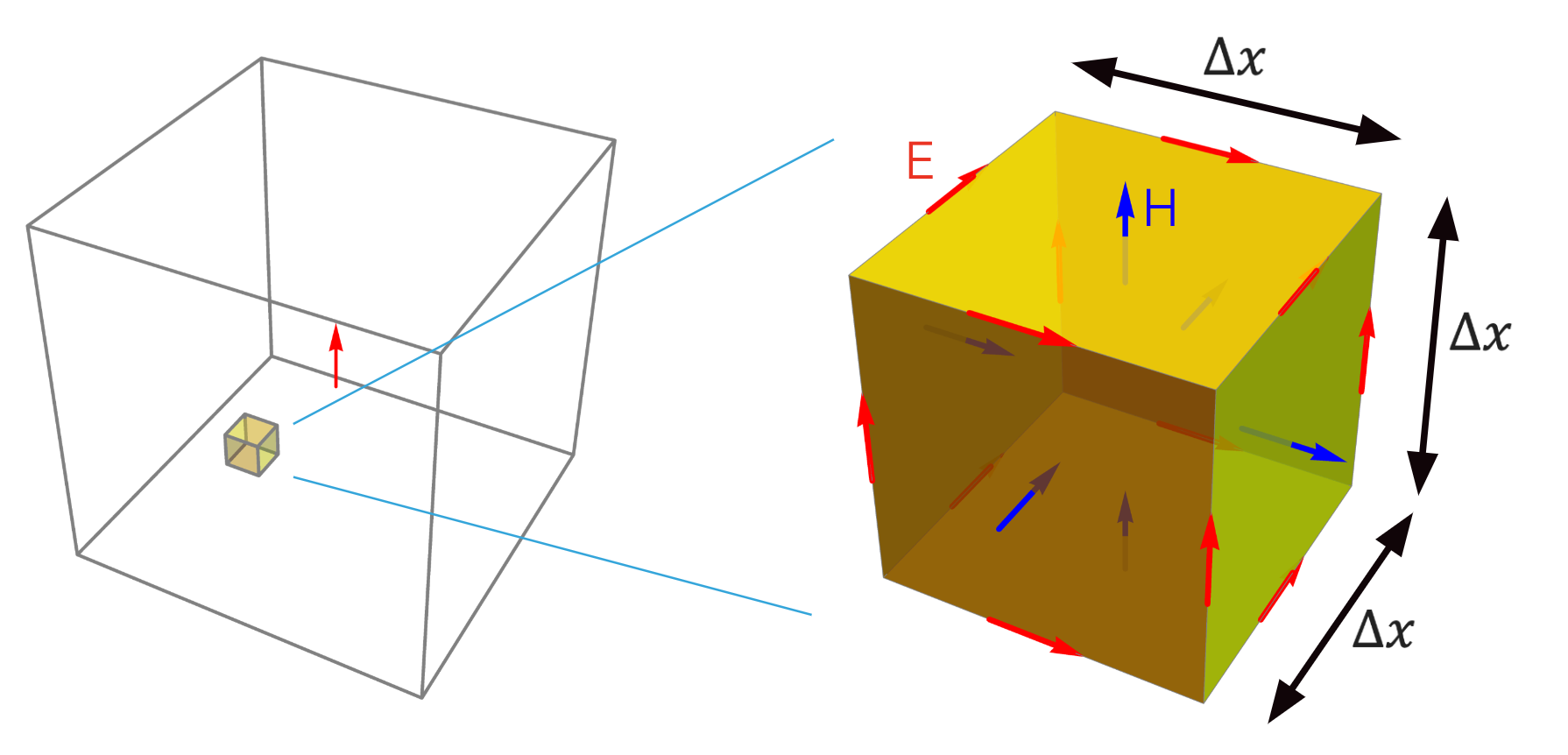
In the finite-difference time domain method, the computational domain is discretized by a little cubes called the Yee cell. A discrete lattice formed by this Yee cell is used to describe the fields. In 3D, the electric fields are distributed on the edge of the Yee cell and the magnetic fields are distributed on the surface of the Yee cell.

Note

A typical rule of thumb is to choose the discretization to be about \(\frac{\lambda_m}{20}\) where \(\lambda_m\) is the field wavelength.

Numerical Dispersion - 1D Illustration

Numerical dispersion is a form of numerical error dependent on the spatial and temporal discretization of the fields. In order to reduce it, it is necessary to improve the discretization of the simulation for particular frequencies and spatial features. This is an important aspect of defining the grid.

Consider a standard 1D wave equation in vacuum:

\[\left( \frac{\delta ^2 }{\delta x^2} - \frac{1}{c^2} \frac{\delta^2}{\delta t^2} \right) E = 0\]

which is ideally solved into a monochromatic travelling wave:

\[E(x) = e^{j (kx - \omega t)}\]

This physical wave is described with a wavevector \(k\) for the spatial field variations and the angular frequency \(\omega\) for temporal field variations. The spatial and temporal field variations are related by a dispersion relation.

The ideal dispersion relation is:

\[\left( \frac{\omega}{c} \right)^2 = k^2\]

However, in the FDTD simulation, the spatial and temporal fields are discrete.

The same 1D monochromatic wave can be solved using the FDTD method where \(m\) is the index in the grid:

\[\frac{\delta^2}{\delta x^2} E(x_i) \approx \frac{1}{\Delta x^2} \left[ E(x_i + \Delta x) + E(x_i - \Delta x) - 2 E(x_i) \right]\]

\[\frac{\delta^2}{\delta t^2} E(t_{\alpha}) \approx \frac{1}{\Delta t^2} \left[ E(t_{\alpha} + \Delta t) + E(t_{\alpha} - \Delta t) - 2 E(t_{\alpha}) \right]\]

Hence, these discrete fields have this new dispersion relation:

\[\left( \frac{1}{c \Delta t} \text{sin} \left( \frac{\omega \Delta t}{2} \right)^2 \right) = \left( \frac{1}{\Delta x} \text{sin} \left( \frac{k \Delta x}{2} \right) \right)^2\]

The ideal wave solution and the discrete solution have a mismatch illustrated below as a result of the numerical error introduced by numerical dispersion. This plot illustrates the angular frequency as a function of wavevector for both the physical ideal wave and the numerical discrete wave implemented in FDTD.

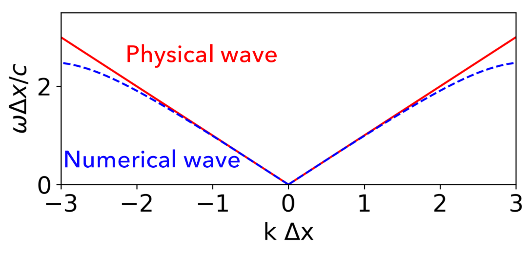
At lower frequencies, when the discretization of \(\Delta x\) is small compared to the wavelength the error between the solutions is very low. When this proportionality increases between the spatial step size and the angular wavelength, this introduces numerical dispersion errors.

\[k \Delta x = \frac{2 \pi}{\lambda_k} \Delta x\]

Usage Recommendations

• It is important to understand the relationship between the time-step \(\Delta t\) defined by the courant factor, and the spatial grid distribution to guarantee simulation stability.

• If your structure has small features, consider using a spatially nonuniform grid. This guarantees finer spatial resolution near the features, but away from it you use have a larger (and computationally faster) grid. In this case, the time step \(\Delta t\) is defined by the smallest spatial grid size.

See also

courant

The Courant-Friedrichs-Lewy (CFL) stability factor

GridSpec

Collective grid specification for all three dimensions.

UniformGrid

Uniform 1D grid.

AutoGrid

Specification for non-uniform grid along a given dimension.

Notebooks:

• Using automatic nonuniform meshing

Lectures:

• Time step size and CFL condition in FDTD

• Numerical dispersion in FDTD

medium

Background medium of simulation, defaults to vacuum if not specified.

See also

Material Library:

The material library is a dictionary containing various dispersive models from real world materials.

Index:

Dispersive and dispersionless Mediums models.

Notebooks:

• Fitting dispersive material models

Lectures:

• Modeling dispersive material in FDTD

GUI:

• Mediums

normalize_index

Index of the source in the tuple of sources whose spectrum will be used to normalize the frequency-dependent data. If None, the raw field data is returned. If None, the raw field data is returned unnormalized.

monitors

Tuple of monitors in the simulation. Monitor names are used to access data after simulation is run.

See also

Index

All the monitor implementations.

sources

Tuple of electric current sources injecting fields into the simulation.

Example

Simple application reference:

Simulation(
   ...
   sources=[
       UniformCurrentSource(
           size=(0, 0, 0),
           center=(0, 0.5, 0),
           polarization="Hx",
           source_time=GaussianPulse(
               freq0=2e14,
               fwidth=4e13,
           ),
       )
   ],
   ...
)

See also

Index:

Frequency and time domain source models.

shutoff

Ratio of the instantaneous integrated E-field intensity to the maximum value at which the simulation will automatically terminate time stepping. Used to prevent extraneous run time of simulations with fully decayed fields. Set to 0 to disable this feature.

structures

Tuple of structures present in simulation. Structures defined later in this list override the simulation material properties in regions of spatial overlap.

Example

Simple application reference:

Simulation(
    ...
    structures=[
         Structure(
         geometry=Box(size=(1, 1, 1), center=(0, 0, 0)),
         medium=Medium(permittivity=2.0),
         ),
    ],
    ...
)

Usage Caveats

It is very important to understand the way the dielectric permittivity of the Structure list is resolved by the simulation grid. Without subpixel averaging, the structure geometry in relation to the grid points can lead to its features permittivity not being fully resolved by the simulation.

For example, in the image below, two silicon slabs with thicknesses 150nm and 175nm centered in a grid with spatial discretization \(\Delta z = 25\text{nm}\) will compute equivalently because that grid does not resolve the feature permittivity in between grid points without subpixel averaging.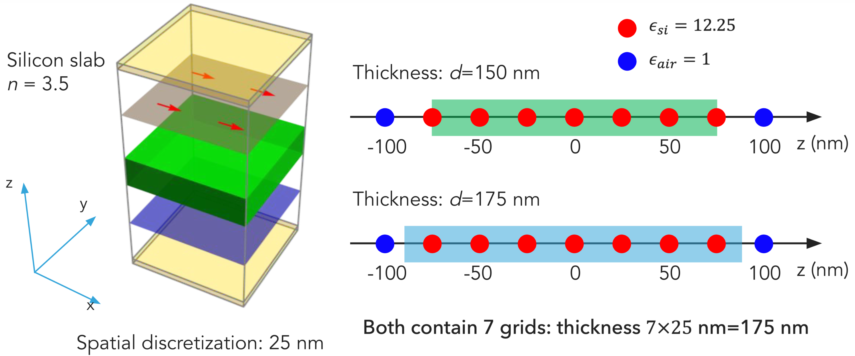

See also

Structure:

Defines a physical object that interacts with the electromagnetic fields.

subpixel

Subpixel averaging of the permittivity based on structure definition, resulting in much higher accuracy for a given grid size.

Notebooks:

• Visualizing geometries in Tidy3D

Lectures:

• Using FDTD to Compute a Transmission Spectrum

• Dielectric constant assignment on Yee grids

GUI:

• Structures

symmetry

You should set the symmetry parameter in your Simulation object using a tuple of integers defining reflection symmetry across a plane bisecting the simulation domain normal to the x-, y-, and z-axis. Each element can be 0 (no symmetry), 1 (even, i.e. PMC symmetry) or -1 (odd, i.e. PEC symmetry). Note that the vectorial nature of the fields must be considered to determine the symmetry value correctly.

The figure below illustrates how the electric and magnetic field components transform under PEC- and PMC-like symmetry planes. You can refer to this figure when considering whether a source field conforms to a PEC- or PMC-like symmetry axis. This would be helpful, especially when dealing with optical waveguide modes.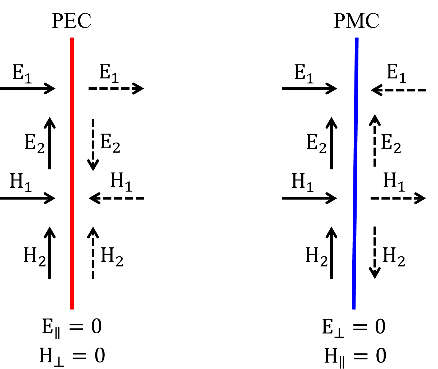

run_time

Total electromagnetic evolution time in seconds. If simulation ‘shutoff’ is specified, simulation will terminate early when shutoff condition met.

How long to run a simulation?

The frequency-domain response obtained in the FDTD simulation only accurately represents the continuous-wave response of the system if the fields at the beginning and at the end of the time stepping are (very close to) zero. So, you should run the simulation for a time enough to allow the electromagnetic fields decay to negligible values within the simulation domain.

When dealing with light propagation in a NON-RESONANT device, like a simple optical waveguide, a good initial guess to simulation run_time would be the a few times the largest domain dimension (\(L\)) multiplied by the waveguide mode group index (\(n_g\)), divided by the speed of light in a vacuum (\(c_0\)), plus the source_time:

\[t_{sim} \approx \frac{n_g L}{c_0} + t_{source}\]

By default, tidy3d checks periodically the total field intensity left in the simulation, and compares that to the maximum total field intensity recorded at previous times. If it is found that the ratio of these two values is smaller than the default shutoff value \(10^{-5}\), the simulation is terminated as the fields remaining in the simulation are deemed negligible. The shutoff value can be controlled using the shutoff parameter, or completely turned off by setting it to zero. In most cases, the default behavior ensures that results are correct, while avoiding unnecessarily long run times. The Flex Unit cost of the simulation is also proportionally scaled down when early termination is encountered.

Resonant Caveats

Should I make sure that fields have fully decayed by the end of the simulation?

The main use case in which you may want to ignore the field decay warning is when you have high-Q modes in your simulation that would require an extremely long run time to decay. In that case, you can use the the tidy3d.plugins.resonance.ResonanceFinder plugin to analyze the modes, as well as field monitors with vaporization to capture the modal profiles. The only thing to note is that the normalization of these modal profiles would be arbitrary, and would depend on the exact run time and apodization definition. An example of such a use case is presented in our case study.

See also

Notebooks

• High-Q silicon resonator

classmethod bloch_with_symmetry(val, values)

Error if a Bloch boundary is applied with symmetry

classmethod plane_wave_boundaries(val, values)

Error if there are plane wave sources incompatible with boundary conditions.

classmethod bloch_boundaries_diff_mnt(val, values)

Error if there are diffraction monitors incompatible with boundary conditions.

classmethod tfsf_boundaries(val, values)

Error if the boundary conditions are compatible with TFSF sources, if any.

classmethod tfsf_with_symmetry(val, values)

Error if a TFSF source is applied with symmetry

classmethod check_fixed_angle_components(values)

Error if a fixed-angle plane wave is combined with other sources or fully anisotropic mediums or gain mediums.

classmethod boundaries_for_zero_dims(val, values)

Error if absorbing boundaries, bloch boundaries, unmatching pec/pmc, or symmetry is used along a zero dimension.

classmethod diffraction_monitor_boundaries(val, values)

If any DiffractionMonitor exists, ensure boundary conditions in the transverse directions are periodic or Bloch.

classmethod proj_distance_for_approx(val, values)

Warn if projection distance for projection monitors is not large compared to monitor or, simulation size, yet far_field_approx is True.

classmethod diffraction_monitor_medium(val, values)

If any DiffractionMonitor exists, ensure is does not lie in a lossy medium.

validate_pre_upload(source_required=True)

Validate the fully initialized simulation is ok for upload to our servers.

Parameters:

source_required (bool = True) – If True, validation will fail in case no sources are found in the simulation.

property monitors_data_size

Dictionary mapping monitor names to their estimated storage size in bytes.

with_adjoint_monitors(sim_fields_keys)

Copy of self with adjoint field and permittivity monitors for every traced structure.

make_adjoint_monitors(sim_fields_keys)

Get lists of field and permittivity monitors for this simulation.

property freqs_adjoint

Unique list of all frequencies. For now should be only one.

property mediums

Returns set of distinct AbstractMedium in simulation.

Returns:

Set of distinct mediums in the simulation.

Return type:

List[AbstractMedium]

property medium_map

Returns dict mapping medium to index in material. medium_map[medium] returns unique global index of AbstractMedium in simulation.

Returns:

Mapping between distinct mediums to index in simulation.

Return type:

Dict[AbstractMedium, int]

property background_structure

Returns structure representing the background of the Simulation.

static intersecting_media(test_object, structures)

From a given list of structures, returns a list of AbstractMedium associated with those structures that intersect with the test_object, if it is a surface, or its surfaces, if it is a volume.

Parameters:

• test_object (Box) – Object for which intersecting media are to be detected.

• structures (List[AbstractMedium]) – List of structures whose media will be tested.

Returns:

Set of distinct mediums that intersect with the given planar object.

Return type:

List[AbstractMedium]

static intersecting_structures(test_object, structures)

From a given list of structures, returns a list of Structure that intersect with the test_object, if it is a surface, or its surfaces, if it is a volume.

Parameters:

• test_object (Box) – Object for which intersecting media are to be detected.

• structures (List[AbstractMedium]) – List of structures whose media will be tested.

Returns:

Set of distinct structures that intersect with the given surface, or with the surfaces of the given volume.

Return type:

List[Structure]

monitor_medium(monitor)

Return the medium in which the given monitor resides.

Parameters:

monitor (Monitor) – Monitor whose associated medium is to be returned.

Returns:

Medium associated with the given Monitor.

Return type:

AbstractMedium

to_gdstk(x=None, y=None, z=None, permittivity_threshold=1, frequency=0, gds_layer_dtype_map=None)

Convert a simulation’s planar slice to a .gds type polygon list.

Parameters:

• x (float = None) – Position of plane in x direction, only one of x,y,z can be specified to define plane.

• y (float = None) – Position of plane in y direction, only one of x,y,z can be specified to define plane.

• z (float = None) – Position of plane in z direction, only one of x,y,z can be specified to define plane.

• permittivity_threshold (float = 1) – Permittivity value used to define the shape boundaries for structures with custom medim

• frequency (float = 0) – Frequency for permittivity evaluation in case of custom medium (Hz).

• gds_layer_dtype_map (Dict) – Dictionary mapping mediums to GDSII layer and data type tuples.

Returns:

List of gdstk.Polygon.

Return type:

List

to_gdspy(x=None, y=None, z=None, gds_layer_dtype_map=None)

Convert a simulation’s planar slice to a .gds type polygon list.

Parameters:

• x (float = None) – Position of plane in x direction, only one of x,y,z can be specified to define plane.

• y (float = None) – Position of plane in y direction, only one of x,y,z can be specified to define plane.

• z (float = None) – Position of plane in z direction, only one of x,y,z can be specified to define plane.

• gds_layer_dtype_map (Dict) – Dictionary mapping mediums to GDSII layer and data type tuples.

Returns:

List of gdspy.Polygon and gdspy.PolygonSet.

Return type:

List

to_gds(cell, x=None, y=None, z=None, permittivity_threshold=1, frequency=0, gds_layer_dtype_map=None)

Append the simulation structures to a .gds cell.

Parameters:

• cell (gdstk.Cell or gdspy.Cell) – Cell object to which the generated polygons are added.

• x (float = None) – Position of plane in x direction, only one of x,y,z can be specified to define plane.

• y (float = None) – Position of plane in y direction, only one of x,y,z can be specified to define plane.

• z (float = None) – Position of plane in z direction, only one of x,y,z can be specified to define plane.

• permittivity_threshold (float = 1) – Permittivity value used to define the shape boundaries for structures with custom medim

• frequency (float = 0) – Frequency for permittivity evaluation in case of custom medium (Hz).

• gds_layer_dtype_map (Dict) – Dictionary mapping mediums to GDSII layer and data type tuples.

to_gds_file(fname, x=None, y=None, z=None, permittivity_threshold=1, frequency=0, gds_layer_dtype_map=None, gds_cell_name='MAIN')

Append the simulation structures to a .gds cell.

Parameters:

• fname (str) – Full path to the .gds file to save the Simulation slice to.

• x (float = None) – Position of plane in x direction, only one of x,y,z can be specified to define plane.

• y (float = None) – Position of plane in y direction, only one of x,y,z can be specified to define plane.

• z (float = None) – Position of plane in z direction, only one of x,y,z can be specified to define plane.

• permittivity_threshold (float = 1) – Permittivity value used to define the shape boundaries for structures with custom medim

• frequency (float = 0) – Frequency for permittivity evaluation in case of custom medium (Hz).

• gds_layer_dtype_map (Dict) – Dictionary mapping mediums to GDSII layer and data type tuples.

• gds_cell_name (str = 'MAIN') – Name of the cell created in the .gds file to store the geometry.

property frequency_range

Range of frequencies spanning all sources’ frequency dependence.

Returns:

Minimum and maximum frequencies of the power spectrum of the sources.

Return type:

Tuple[float, float]

plot_3d(width=800, height=800)

Render 3D plot of Simulation (in jupyter notebook only). :param width: width of the 3d view dom’s size :type width: float = 800 :param height: height of the 3d view dom’s size :type height: float = 800

property scaled_courant

When conformal mesh is applied, courant number is scaled down depending on conformal_mesh_spec.

property dt

Simulation time step (distance).

Returns:

Time step (seconds).

Return type:

float

property tmesh

FDTD time stepping points.

Returns:

Times (seconds) that the simulation time steps through.

Return type:

np.ndarray

property num_time_steps

Number of time steps in simulation.

__hash__()

Hash method.

property self_structure

The simulation background as a Structure.

property all_structures

List of all structures in the simulation (including the Simulation.medium).

property num_cells

Number of cells in the simulation grid.

Returns:

Number of yee cells in the simulation.

Return type:

int

property num_computational_grid_points

Number of cells in the computational domain for this simulation. This is usually different from num_cells due to the boundary conditions. Specifically, all boundary conditions apart from Periodic require an extra pixel at the end of the simulation domain. On the other hand, if a symmetry is present along a given dimension, only half of the grid cells along that dimension will be in the computational domain.

Returns:

Number of yee cells in the computational domain corresponding to the simulation.

Return type:

int

get_refractive_indices(freq)

List of refractive indices in the simulation at a given frequency. For anisotropic medium, highest refractive index among the 3 main diagonal components is selected.

property n_max

Maximum refractive index in the Simulation.

property wvl_mat_min

Minimum wavelength in the materials present throughout the simulation.

Returns:

Minimum wavelength in the material (microns).

Return type:

float

property complex_fields

Whether complex fields are used in the simulation. Currently this only happens when there are Bloch boundaries.

Returns:

Whether the time-stepping fields are real or complex.

Return type:

bool

property nyquist_step

Maximum number of discrete time steps to keep sampling below Nyquist limit.

Returns:

The largest N such that N * self.dt is below the Nyquist limit.

Return type:

int

property custom_datasets

List of custom datasets for verification purposes. If the list is not empty, then the simulation needs to be exported to hdf5 to store the data.

property allow_gain

True if any of the mediums in the simulation allows gain.

perturbed_mediums_copy(temperature=None, electron_density=None, hole_density=None, interp_method='linear')

Return a copy of the simulation with heat and/or charge data applied to all mediums that have perturbation models specified. That is, such mediums will be replaced with spatially dependent custom mediums that reflect perturbation effects. Any of temperature, electron_density, and hole_density can be None. All provided fields must have identical coords.

Parameters:

• temperature (Union[) –

  SpatialDataArray,

  TriangularGridDataset, TetrahedralGridDataset,

  ] = None Temperature field data.

• electron_density (Union[) –

  SpatialDataArray,

  TriangularGridDataset, TetrahedralGridDataset,

  ] = None Electron density field data.

• hole_density (Union[) –

  SpatialDataArray,

  TriangularGridDataset, TetrahedralGridDataset,

  ] = None Hole density field data.

• interp_method (InterpMethod, optional) – Interpolation method to obtain heat and/or charge values that are not supplied at the Yee grids.

Returns:

Simulation after application of heat and/or charge data.

Return type:

Simulation

classmethod from_scene(scene, **kwargs)

Create a simulation from a Scene instance. Must provide additional parameters to define a valid simulation (for example, run_time, grid_spec, etc).

Parameters:

• scene (Scene) – Size of object in x, y, and z directions.

• **kwargs – Other arguments passed to new simulation instance.

Example

>>> from tidy3d import Scene, Medium, Box, Structure, GridSpec
>>> box = Structure(
...     geometry=Box(center=(0, 0, 0), size=(1, 2, 3)),
...     medium=Medium(permittivity=5),
... )
>>> scene = Scene(
...     structures=[box],
...     medium=Medium(permittivity=3),
... )
>>> sim = Simulation.from_scene(
...     scene=scene,
...     center=(0, 0, 0),
...     size=(5, 6, 7),
...     run_time=1e-12,
...     grid_spec=GridSpec.uniform(dl=0.4),
... )