1.3. Run CFD on a propeller using a Rotation interface
1.3.1. Quick Start using the XV 15 geometry.
The XV15 tiltotor airplane is a commonly used test bed for propeller validation work. As you can see from the following papers, we have done extensive validation work on that geometry. We will now use it to show you how to analyze a propeller-type geometry using a sliding mesh interface. :
1.3.2. Basic description of setup
In order to run a rotating geometry we need to set up a mesh with two blocks, an inner “rotational volume” and an outer “stationary volume”. The interface between those two volumes needs to be a solid of revolution, ie sphere/cylinder/etc…
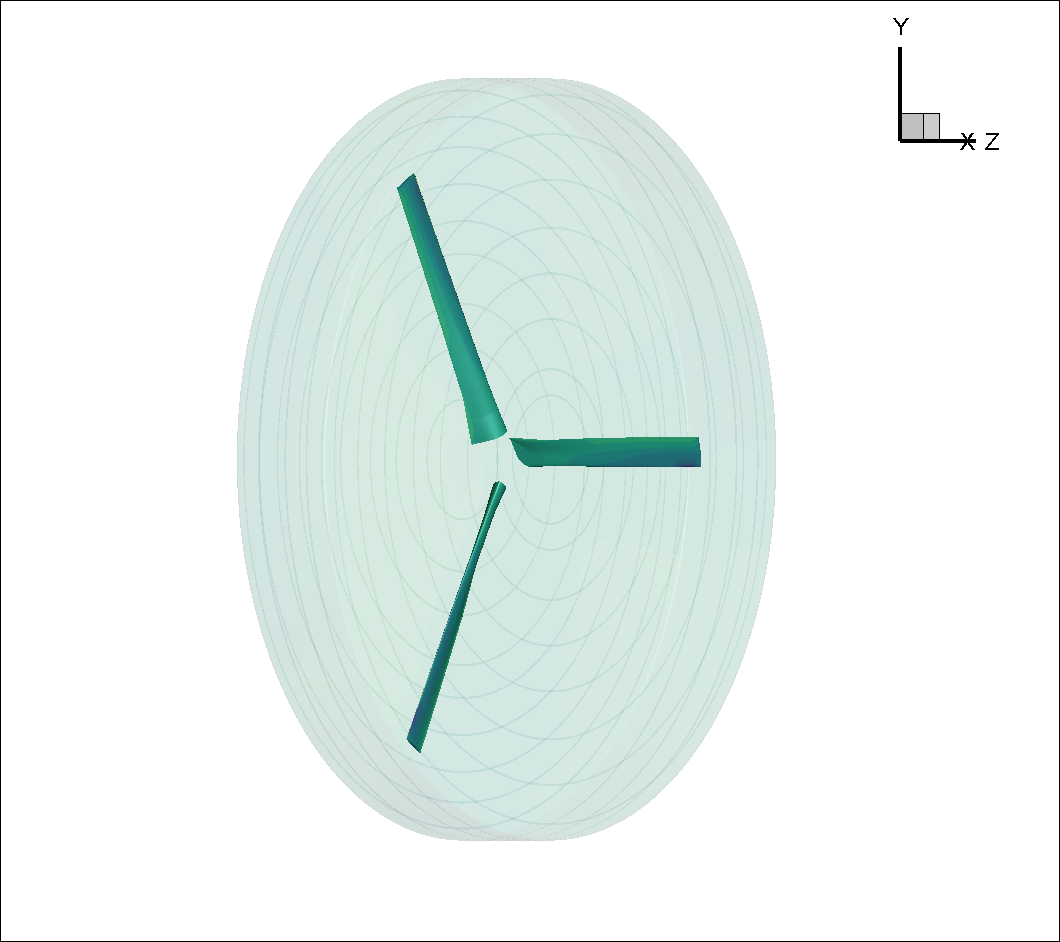
Fig. 1.3.1 Inner block enclosing the XV15 3 bladed prop
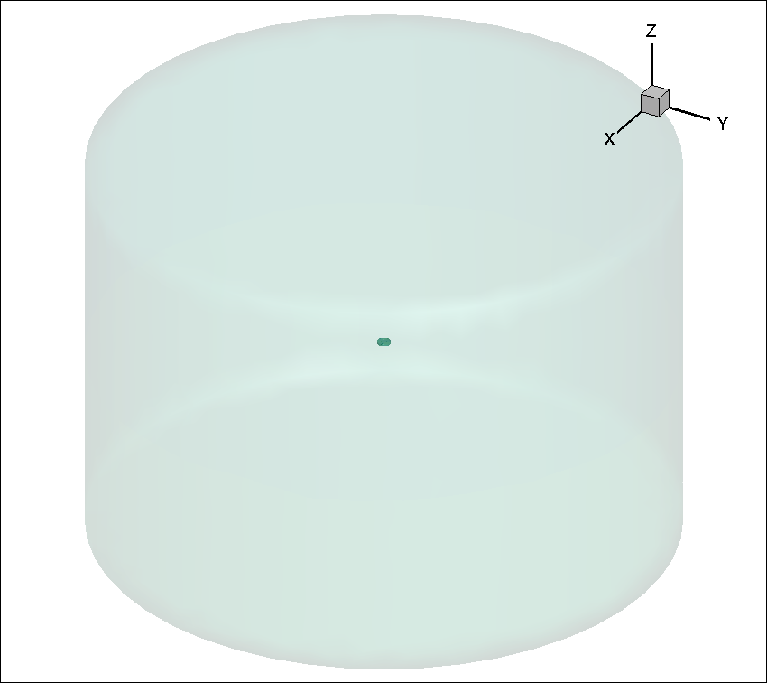
Fig. 1.3.2 Farfield volume enclosing Inner block
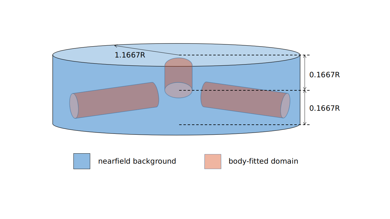
Fig. 1.3.3 body fitted cylinder blocks inside a larger nearfield domain
Please note that it is possible, just like in the figure above, to set up nested rotational interfaces to simulate for example a rotating propeller with blades that pitch as they rotate (i.e. a helicopter's cyclical ). We could also put many rotating blocks inside the stationary farfield block to simulate multiple rotors
1.3.2.1. Rotation interface
The rotation interface needs to be a body of revolution (sphere, cylinder etc…) which encloses the entire rotor blades. The grid points on the rotation interface can not be arbitrary. It is mandatory that they form a set of concentric rings.
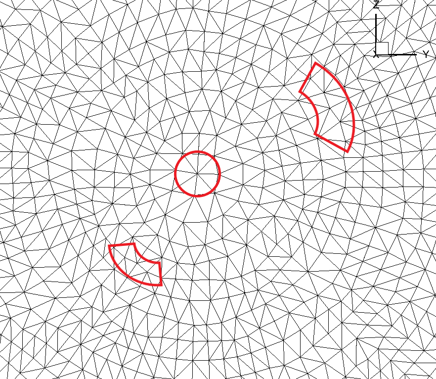
Fig. 1.3.4 Non concentric circle mesh on rotation interface
The grid points on the rotation interface shown in the figure above do not satisfy that requirement. Certain points deviate slightly from the perfect concentric circle.
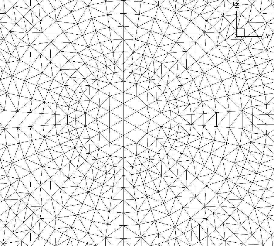
Fig. 1.3.5 Concentric circle mesh on rotation interface
This figure shows a slightly different grid that does satisfy that requirement. Notice how all the nodes are on concentric circles. The reason for that requirement is that it greatly speeds up the interpolation process. Since this interpolation happens twice for every interface node (inner and outer domain) and for every pseudo timestep, already knowing where the neighbors are without having to run a search algorithm every time to find the closest node is very efficient.
1.3.2.2. Creating an interface regions with concentric mesh rings
For this case study we will provide the mesh. But for your own cases, knowing that we have this concentric mesh requirement, the easiest way to create the meshes for the interface regions is to do it programmatically. We have a lot of scripts to generate various body of revolution interface shapes that will allow you to generate an interface region no matter what your geometry. Just contact us and we will help you get setup with the scripts you need.
For plain cylindrical or spherical interfaces we have some pre-generated interfaces in CGNS format ready for you to download from this link. You will notice that they come in various height to radius ratio as well as various resolutions. You will need to choose the version that best fits your needs and then rotate/scale the imported mesh to align the interface around your geometry.
1.3.3. XV15 Example setup
We will now show you how to run an XV15 propeller
First, the rotor has a 150” (inches) radius and the blades have a chord of roughly 11”. For simplicity’s sake we will use the SI system and convert that to 3.81meters radius and 0.279meter chord.
A complete CGNS mesh is available here along with its associated Mesh.json file
if you are comfortable with the CGNS format you can run the “cgnslist” command which will show you that the XV15_Hover_ascent_coarse.cgns file contains the following blocks and boundaries
farField
farField/farField
farField/rotationInterface
innerRotating
innerRotating/blade
innerRotating/rotationInterface
This shows us that we have two mesh regions (farField and innerRotating). Inside innerRotating we have some blades and as a part or farField we have the farField boundaries.
1.3.3.1. Defining a Mesh.json file
The Mesh.json file contains the information the mesh preprocessor needs in order to perform its job. We need to give it the information as to which domains are the “NoSlipWalls” and which are the “rotationInterfaces” along with some key rotation interface geometry information, namely the rotation axis vector and the center of rotation.
You do NOT need to give it any “FarField”, “SlipWall” domain informations.
In our case our XV15_quick_start_mesh.json file looks like:
{
  "boundaries": {
      "noSlipWalls": [
          "innerRotating/blade"]
  },
  "slidingInterfaces" : [
      {
        "stationaryPatches" : ["farField/rotationInterface"],
        "rotatingPatches" : ["innerRotating/rotationInterface"],
          "axisOfRotation" : [0,0,-1],
          "centerOfRotation" : [0,0,0]
      }
  ]
  }
1.3.3.2. Uploading your mesh
Now that you have the XV15_Hover_ascent_coarse.cgns mesh file and its associated XV15_quick_start_mesh.json mesh preprocessor input file you can upload your mesh either using the API or by using the web UI
1.3.3.3. Defining a Flow360.json file.
Once your mesh has been uploaded, the last step before launching a run is to create a Flow360.json file with all the information needed by Flow360 to run your case.
For this example we have provided you with two different Flow360 json input files. Please download the one for the initial 1st order run and the other for the final 2nd order runs. More on 1st order vs 2nd order below
For this case, our Flow360 input json files have 11 sections
“geometry”
“runControl”
“volumeOutput”
“surfaceOutput”
“sliceOutput”
“navierStokesSolver”
“turbulenceModelSolver”
“freestream”
“boundaries”
“slidingInterfaces”
“timeStepping”
Most of those categories are self evident and won’t be discussed here, just take a look at the downloaded json files or go to our documentation page on solver configuration to see what each sections does. Or for a more detailed description on how to setup your Flow360.json file for your configuration please see our dedicated Case Studies
1.3.3.4. 1st vs 2nd order CFD runs:
IF you look at the Flow360.json files you will see something like:
“navierStokesSolver” : {
“orderOfAccuracy” : 1 or 2 }
“turbulenceModelSolver” : {
“orderOfAccuracy” : 1 or 2 }
This dictates whether the code will run using 1st or 2nd order interpolation in space algorithms. 1st order accuracy is much faster and much more robust.
For time accurate runs where we have rotating components we recommend to first run 1 revolution using first order “orderOfAccuracy” to help establish the flow. Then follow that with however many 2nd order accurate revolutions are needed for the flow to properly establish itself and for the forces to stabilize. Please note that if you have some parts of your vehicle downstream of your propellers it may take many revolutions for the propeller’s wake to reach the downstream geometry components. If that is the case you could run a first set of 2nd order accurate revolutions with a larger time step to help the flow establish itself quicker and then do a more precise, better converged, 2nd order run with smaller time steps to get more accurate forces. This is easily done in Flow360 through our “fork” function that launches a new job using the flow solution of the parent job as the initial condition to the forked child job.
Also, for 1st order we recommend using the following “timeStepping” values:
max Pseudo Steps =12
CFL initial=1
CFL final = 1000
rampSteps= 10 (i.e. rampSteps is 2 steps less then maxPseudoSteps)
for 2nd order we recommend using the following “timeStepping” values:
max Pseudo Steps =35
CFL initial=1
CFL final = 1e7
rampSteps= 33 (i.e. rampSteps is 2 steps less then maxPseudoSteps)
These are just guidelines to get your started and will most likely need to be revised for your specific cases.
1.3.3.5. Case input conditions
For our case we have the following input conditions:
5m/s inflow speed
600 RPM
speed of sound = 340.2 m/s
Rho = 1.225 kg/m3
Alpha = -90 ° which means the air coming down from above, i.e. an ascent case.
other key values are :
The reference Mach value is arbitrarily set to the Tip mach number for the blades.
For the 1st order run we will do 1 revolution at 6 ° per time step. Hence the “maxPhysicalSteps” : 60 value (60*6 ° =360 ° )
for the 2nd order run we will do 5 revolutions at 3 ° per time step.
Using the Non-dimensionalization equations described in the conventions part of the documentation we get the following flow conditions and timeStepping values in our 1st order Flow360.json file.
{    "freestream" :
    {
        "muRef" : 4.29279e-08,
        "Mach" : 1.46972e-02,
        "MachRef" : 0.70,
        "Temperature" : 288.15,
        "alphaAngle" : -90.0,
        "betaAngle" : 0.0
    },
    "boundaries" : {
        "farField/farField" : { "type" : "Freestream" },
        "farField/rotationInterface" : { "type" : "SlidingInterface" },
        "innerRotating/rotationInterface" :   { "type" : "SlidingInterface" },
        "innerRotating/blade" :   { "type" : "NoSlipWall" }
    },
    "slidingInterfaces" : [
    {
        "stationaryPatches" : ["farField/rotationInterface"],
        "rotatingPatches" : ["innerRotating/rotationInterface"],
        "axisOfRotation" : [0,0,-1],
        "centerOfRotation" : [0,0,0],
        "omega" : 1.84691e-01,
        "volumeName" : ["innerRotating"]
    }
    ],
    "timeStepping" : {
              "timeStepSize" : 5.67000e-01,
              "maxPhysicalSteps" : 60,
              "maxPseudoSteps" : 12,
        "CFL" : {
            "initial" : 1,
            "final" : 1000,
            "rampSteps" : 10
        }
    }
    }
1.3.3.6. Case running
The first order case should finish in less then a minute on this fairly coarse 915K node mesh.
The second order run takes about 3.5 to 4 minutes to run its 5 revolutions. Please note that at the end of the 2nd order run you will have done 6 revolutions (1 for the 1st order run and 5 for the 2nd order run).
For a time accurate case to be considered well converged we like to have at least 2 orders of magnitude in the residuals within each time step.
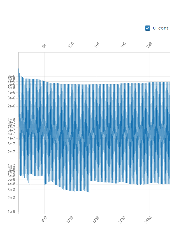
Fig. 1.3.6 2nd order convergence plot showing more then 2 orders of magnitude decrease in the residuals for each subiterations.
The forces also seem to have stabilized after running for 6 revolutions
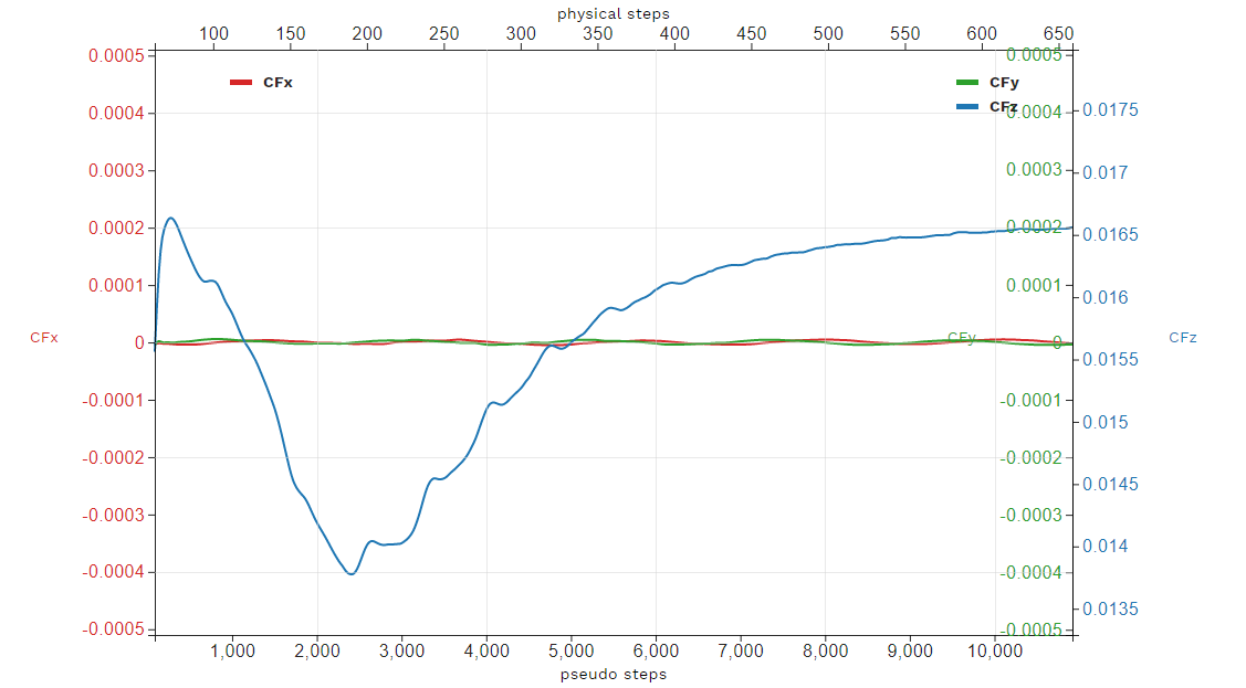
Fig. 1.3.7 2nd order run’s force history plot showing good stabilization of the forces.
Congratulations. You have now run your first propeller using a rotational interface in Flow360.