Inverse design optimization of a compact grating coupler
Contents
Inverse design optimization of a compact grating coupler#
This notebook contains a long optimization. Running the entire notebook will cost about 20 FlexCredits and take several hours.
The ability to couple light in and out of photonic integrated circuits (PICs) is crucial for developing wafer-scale systems and tests. This need makes designing efficient and compact grating couplers an important task in the PIC development cycle. In this notebook, we will demonstrate how to use Tidy3D’s adjoint plugin to perform the inverse design of a compact 3D grating coupler. We will show how to improve design fabricability by enhancing permittivity binarization and controlling the device’s minimum feature size.
We start by importing our typical python packages, jax, tidy3d and its adjoint plugin.
[1]:
# Standard python imports.
from typing import List
import numpy as np
import scipy as sp
import matplotlib.pylab as plt
import os
import json
import pydantic as pd
from typing import Callable

# Import jax to be able to use automatic differentiation.
import jax.numpy as jnp
import jax.scipy as jsp
from jax import value_and_grad

# Import regular tidy3d.
import tidy3d as td
import tidy3d.web as web

# Import the components we need from the adjoint plugin.
from tidy3d.plugins.adjoint import (
    JaxSimulation,
    JaxBox,
    JaxCustomMedium,
    JaxStructure,
    JaxSimulationData,
    JaxDataArray,
    JaxPermittivityDataset,
)
from tidy3d.plugins.adjoint.web import run
Grating Coupler Inverse Design Configuration#
The grating coupler inverse design begins with a rectangular design region connected to a \(Si\) waveguide. Throughout the optimization process, this initial structure evolves to convert a vertically incident Gaussian-like mode from an optical fiber into a guided mode and then funnel it into the \(Si\) waveguide.
We are considering a full-etched grating structure, so a \(SiO_{2}\) BOX layer is included. To reduce backreflection, we adjusted the fiber tilt angle to \(10^{\circ}\) [1, 2].
In the following block of code, you can find the parameters that can be modified to configure the grating coupler structure, optimization, and simulation setup. Special care should be devoted to the it_per_step and opt_steps variables bellow.
[2]:
# Geometric parameters.
w_thick = 0.22  # Waveguide thickness (um).
w_width = 0.5  # Waveguide width (um).
w_length = 1.0  # Waveguide length (um).
box_thick = 1.6  # SiO2 BOX thickness (um).
spot_size = 2.5  # Spot size of the input Gaussian field regarding a lensed fiber (um).
fiber_tilt = 10.0  # Fiber tilt angle (degrees).
src_offset = 0.05  # Distance between the source focus and device (um).

# Material.
nSi = 3.48  # Silicon refractive index.
nSiO2 = 1.44  # Silica refractive index.

# Design region parameters.
gc_width = 4.0  # Grating coupler width (um).
gc_length = 4.0  # Grating coupler length (um).
dr_grid_size = 0.02  # Grid size within the design region (um).

# Inverse design set up parameters.
#################################################################
# Total number of iterations = opt_steps x it_per_step.
it_per_step = 10  # Number of iterations per optimization step.
opt_steps = 15 # Number of optimization steps.
#################################################################
feature_size = 0.070 # Minimum feature size (um).
eta = 0.50  # Threshold value for the projection filter.
init_beta = 10  # Sharpness parameter for the projection filter.
del_beta = 10  # Increments of beta at each optimization step.
fom_name = "fom_field"  # Name of the monitor used to compute the objective function.

# Inverse design data file.
output_file = "./misc/invdes_gc.json"

# Simulation wavelength.
wl = 1.55  # Central simulation wavelength (um).
bw = 0.06  # Simulation bandwidth (um).
n_wl = 61  # Number of wavelength points within the bandwidth.
Ckeching For a Previous Optimization#
If output_file is a valid file, the results of a previous optimization are loaded, then the optimization will continue from the last iteration step. If the optimization was completed, only the final structure will be simulated. The JSON file used in this notebook can be downloaded from our documentation repo.
[3]:
total_iter = opt_steps * it_per_step
iter_to_do = total_iter
prev_data = []
if os.path.isfile(output_file):
    with open(output_file, "r", encoding="utf-8") as json_file:
        prev_data = json.load(json_file)[0]
        iter_to_do -= len(prev_data["obj_vals"])
        print("Previous optimization data loaded from " + output_file)

print(f"Total iterations = {total_iter}")
print(f"Iterations to run = {iter_to_do}")
Total iterations = 150
Iterations to run = 150
Inverse Design Optimization Set Up#
We will calculate the values of some parameters used throughout the inverse design set up.
[4]:
# Minimum and maximum values for the permittivities.
eps_max = nSi**2
eps_min = 1.0

# Material definitions.
mat_si = td.Medium(permittivity=eps_max)  # Waveguide material.
mat_sio2 = td.Medium(permittivity=nSiO2**2)  # Substrate material.

# Wavelengths and frequencies.
wl_max = wl + bw / 2
wl_min = wl - bw / 2
wl_range = np.linspace(wl_min, wl_max, n_wl)
freq = td.C_0 / wl
freqs = td.C_0 / wl_range
freqw = 0.5 * (freqs[0] - freqs[-1])
run_time = 5e-12

# Computational domain size.
pml_spacing = 0.6 * wl
size_x = pml_spacing + w_length + gc_length
size_y = gc_width + 2 * pml_spacing
size_z = w_thick + box_thick + 2 * pml_spacing
center_z = size_z / 2 - pml_spacing - w_thick / 2
eff_inf = 1000

# Inverse design variables.
src_pos_z = w_thick / 2 + src_offset
mon_pos_x = -size_x / 2 + 0.25 * wl
mon_w = int(3 * w_width / dr_grid_size) * dr_grid_size
mon_h = int(5 * w_thick / dr_grid_size) * dr_grid_size
nx = int(gc_length / dr_grid_size)
ny = int(gc_width / dr_grid_size / 2.0)
npar = nx * ny
dr_size_x = nx * dr_grid_size
dr_size_y = 2 * ny * dr_grid_size
dr_center_x = -size_x / 2 + w_length + dr_size_x / 2
First, we will introduce the simulation components that do not change during optimization, such as the \(Si\) waveguide and \(SiO_{2}\) BOX layer. Additionally, we will include a Gaussian source to drive the simulations, and a mode monitor to compute the objective function.
[5]:
# Input/output waveguide.
waveguide = td.Structure(
    geometry=td.Box.from_bounds(
        rmin=(-eff_inf, -w_width / 2, -w_thick / 2),
        rmax=(-size_x / 2 + w_length, w_width / 2, w_thick / 2),
    ),
    medium=mat_si,
)

# SiO2 BOX layer.
sio2_substrate = td.Structure(
    geometry=td.Box.from_bounds(
        rmin=(-eff_inf, -eff_inf, -w_thick / 2 - box_thick),
        rmax=(eff_inf, eff_inf, -w_thick / 2)
    ),
    medium=mat_sio2,
)

# Si substrate.
si_substrate = td.Structure(
    geometry=td.Box.from_bounds(
        rmin=(-eff_inf, -eff_inf, -eff_inf),
        rmax=(eff_inf, eff_inf, -w_thick / 2 - box_thick)
    ),
    medium=mat_si,
)

# Gaussian source focused above the grating coupler.
gauss_source = td.GaussianBeam(
    center=(dr_center_x, 0, src_pos_z),
    size=(dr_size_x, dr_size_y, 0),
    source_time=td.GaussianPulse(freq0=freq, fwidth=freqw),
    pol_angle=np.pi / 2,
    angle_theta=fiber_tilt * np.pi / 180.0,
    direction="-",
    num_freqs=7,
    waist_radius=spot_size / 2,
)

# Monitor where we will compute the objective function from.
mode_spec = td.ModeSpec(num_modes=1, target_neff=nSi)
fom_monitor = td.ModeMonitor(
    center=[mon_pos_x, 0, 0],
    size=[0, mon_w, mon_h],
    freqs=[freq],
    mode_spec=mode_spec,
    name=fom_name,
)
Now, we will define a random vector of initial design parameters or load a previously designed structure.
[6]:
init_par = np.random.uniform(0, 1, npar)

# Load parameters if continuing/visualizing a previous optimization:
if iter_to_do < total_iter:
    init_par = np.array(prev_data["design_parameters"])
    init_beta = prev_data["final_beta"]
# Only smooths the initial random distribution otherwise.
else:
    init_par = sp.ndimage.gaussian_filter(init_par, 1)
Fabricability Improvements#
We will use jax to build functions that improve device fabricability. A classical conic density filter, which is popular in topology optimization problems, is used to enforce a minimum feature size specified by the feature_size variable. Next, a hyperbolic tangent projection function is applied to eliminate grayscale and obtain a binarized permittivity pattern. The beta parameter controls the sharpness of the transition in the projection function, and for better results, this
parameter should be gradually increased throughout the optimization process. Finally, the design parameters are transformed into permittivity values. For a detailed review of these methods, refer to [3].
[7]:
def get_eps(design_param, beta: float = 1.00, binarize: bool = False) -> np.ndarray:
    """Returns the permittivities after applying a conic density filter on design parameters
    to enforce fabrication constraints, followed by a binarization projection function
    which reduces grayscale.
    Parameters:
        design_param: np.ndarray
            Vector of design parameters.
        beta: float = 1.0
            Sharpness parameter for the projection filter.
        binarize: bool = False
            Enforce binarization.
    Returns:
        eps: np.ndarray
            Permittivity vector.
    """
    # Reshapes the design parameters into a 2D matrix.
    rho = np.reshape(design_param, (nx, ny))

    # Builds the conic filter and apply it to design parameters.
    filter_radius = np.ceil((feature_size * np.sqrt(3)) / dr_grid_size)
    xy = np.linspace(-filter_radius, filter_radius, int(2 * filter_radius + 1))
    xm, ym = np.meshgrid(xy, xy)
    xy_rad = np.sqrt(xm**2 + ym**2)
    kernel = jnp.where(filter_radius - xy_rad > 0, filter_radius - xy_rad, 0)
    filt_den = jsp.signal.convolve(jnp.ones_like(rho), kernel, mode="same")
    rho_dot = jsp.signal.convolve(rho, kernel, mode="same") / filt_den

    # Applies a hyperbolic tangent binarization function.
    rho_bar = (jnp.tanh(beta * eta) + jnp.tanh(beta * (rho_dot - eta))) / (
        jnp.tanh(beta * eta) + jnp.tanh(beta * (1.0 - eta))
    )

    # Calculates the permittivities from the transformed design parameters.
    eps = eps_min + (eps_max - eps_min) * rho_bar
    if binarize:
        eps = jnp.where(eps < (eps_min + eps_max) / 2, eps_min, eps_max)
    else:
        eps = jnp.where(eps < eps_min, eps_min, eps)
        eps = jnp.where(eps > eps_max, eps_max, eps)
    return eps
The permittivity values obtained from the design parameters are then used to build a JaxCustomMedium. As we will consider symmetry about the x-axis in the simulations, only the upper-half part of the design region needs to be populated. A JaxStructure built using the JaxCustomMedium will be returned by the following function:
[8]:
def update_design(eps, unfold: bool = False) -> List[JaxStructure]:
    # Reflects the structure about the x-axis.
    nyii = ny
    y_min = 0
    dr_s_y = dr_size_y / 2
    dr_c_y = dr_s_y / 2
    eps_val = jnp.array(eps).reshape((nx, ny, 1, 1))
    if unfold:
        nyii = 2 * ny
        y_min = -dr_size_y / 2
        dr_s_y = dr_size_y
        dr_c_y = 0
        eps_val = np.concatenate((np.fliplr(np.copy(eps_val)), eps_val), axis=1)

    # Definition of the coordinates x,y along the design region.
    coords_x = [(dr_center_x - dr_size_x / 2) + ix * dr_grid_size for ix in range(nx)]
    coords_y = [y_min + iy * dr_grid_size for iy in range(nyii)]
    coords = dict(x=coords_x, y=coords_y, z=[0], f=[freq])

    # Creation of a custom medium using the values of the design parameters.
    eps_components = {
        f"eps_{dim}{dim}": JaxDataArray(values=eps_val, coords=coords) for dim in "xyz"
    }
    eps_dataset = JaxPermittivityDataset(**eps_components)
    eps_medium = JaxCustomMedium(eps_dataset=eps_dataset)
    box = JaxBox(center=(dr_center_x, dr_c_y, 0), size=(dr_size_x, dr_s_y, w_thick))
    design_structure = JaxStructure(geometry=box, medium=eps_medium)
    return [design_structure]
Next, we will write a function to return the JaxSimulation object. Note that we are using a MeshOverrideStructure to obtain a uniform mesh over the design region.
[9]:
def make_adjoint_sim(
    design_param, beta: float = 1.00, unfold: bool = False, binarize: bool=False
) -> JaxSimulation:
    # Builds the design region from the design parameters.
    eps = get_eps(design_param, beta, binarize)
    design_structure = update_design(eps, unfold=unfold)

    # Creates a uniform mesh for the design region.
    adjoint_dr_mesh = td.MeshOverrideStructure(
        geometry=td.Box(
            center=(dr_center_x, 0, 0), size=(dr_size_x, dr_size_y, w_thick)
        ),
        dl=[dr_grid_size, dr_grid_size, dr_grid_size],
        enforce=True,
    )

    return JaxSimulation(
        size=[size_x, size_y, size_z],
        center=[0, 0, -center_z],
        grid_spec=td.GridSpec.auto(
            wavelength=wl_max,
            min_steps_per_wvl=15,
            override_structures=[adjoint_dr_mesh],
        ),
        symmetry=(0, -1, 0),
        structures=[waveguide, sio2_substrate, si_substrate],
        input_structures=design_structure,
        sources=[gauss_source],
        monitors=[],
        output_monitors=[fom_monitor],
        run_time=run_time,
        subpixel=True,
    )
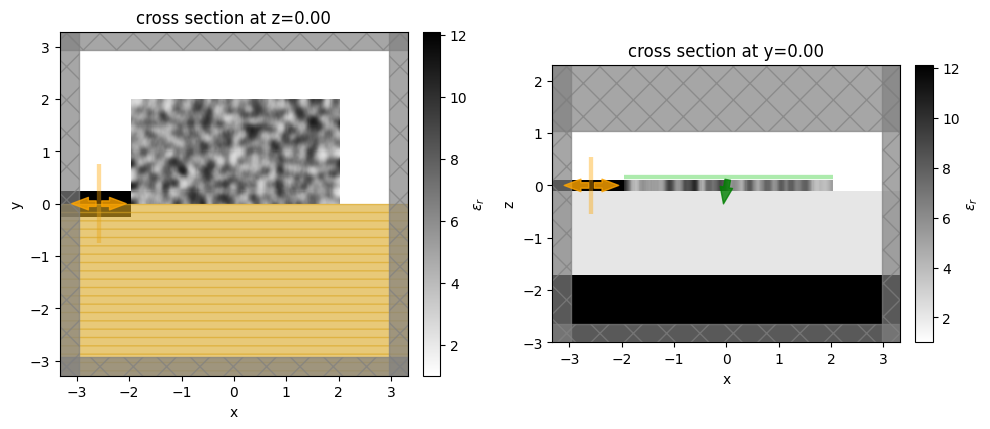
Let’s visualize the simulation set up and verify if all the elements are in their correct places.
[10]:
init_design = make_adjoint_sim(init_par, beta=init_beta)

fig, (ax1, ax2) = plt.subplots(1, 2, tight_layout=True, figsize=(10, 10))
init_design.plot_eps(z=0, ax=ax1)
init_design.plot_eps(y=0, ax=ax2)
plt.show()
WARNING:jax._src.lib.xla_bridge:No GPU/TPU found, falling back to CPU. (Set TF_CPP_MIN_LOG_LEVEL=0 and rerun for more info.)
Optimization#
We need to provide an objective function and its gradients with respect to the design parameters of the optimization algorithm.
Our figure-of-merit (FOM) is the coupling efficiency of the incident power into the fundamental transverse electric mode of the \(Si\) waveguide. The optimization algorithm will call the objective function at each iteration step. Therefore, the objective function will create the adjoint simulation, run it, and return the FOM value.
[11]:
# Figure of Merit (FOM) calculation.
def fom(sim_data: JaxSimulationData) -> float:
    """Return the power at the mode index of interest."""
    output_amps = sim_data.output_data[0].amps
    amp = output_amps.sel(direction="-", f=freq, mode_index=0)
    return jnp.sum(jnp.abs(amp) ** 2)


# Objective function to be passed to the optimization algorithm.
def obj(
    design_param, beta: float = 1.0, step_num: int = None, verbose: bool = False
) -> float:
    sim = make_adjoint_sim(design_param, beta)
    task_name = "inv_des"
    if step_num:
        task_name += f"_step_{step_num}"
    sim_data = run(sim, task_name=task_name, verbose=verbose)
    fom_val = fom(sim_data)
    return fom_val

# Function to calculate the objective function value and its
# gradient with respect to the design parameters.
obj_grad = value_and_grad(obj)
Next, we will define an Optimizer class based on Adam gradient-descent algorithm to drive the inverse design process.
[12]:
class Optimizer(pd.BaseModel):
    class Config:
        arbitrary_types_allowed = True

    val_and_grad: Callable = None # optimization function
    parameters: np.ndarray # current state of the parameters

    # General optimizer.
    objective_history: list = []
    param_history: list = []
    num_it: int = 0 # current iteration number

class AdamOptimizer(Optimizer):
    # Adam specific.
    step_size: float = 0.02
    beta1: float = 0.9
    beta2: float = 0.999
    epsilon: float = 1e-8

    # Adam specific history parameters.
    mt: np.ndarray = None
    vt: np.ndarray = None
    mt_history: list = []
    vt_history: list = []

    def __init__(self,
                init_mt: np.ndarray=None,
                init_vt: np.ndarray=None,
                *args,
                **kwargs):

        super().__init__(*args, **kwargs)
        # Set mt and vt.
        self.mt = np.zeros_like(self.parameters) if init_mt is None else init_mt
        self.vt = np.zeros_like(self.parameters) if init_mt is None else init_vt

    def step(self, *args, **kwargs):
        """args and kwargs are optional extra arguments passed to self.val_and_grad"""

        val, grad = self.val_and_grad(self.parameters, *args, **kwargs)
        grad = np.array(grad).reshape(self.parameters.shape)

        # Display current status and update history variables.
        print(f"At iteration {self.num_it}")
        print(f"\tObjective function = {val:.4e}")
        print(f"\tGrad_norm = {np.linalg.norm(grad):.4e}")

        # Update Adam optimizer history.
        self.num_it += 1
        self.mt = self.beta1 * self.mt + (1 - self.beta1) * grad
        self.vt = self.beta2 * self.vt + (1 - self.beta2) * grad ** 2
        mt_hat = self.mt / (1 - self.beta1 ** self.num_it)
        vt_hat = self.vt / (1 - self.beta2 ** self.num_it)

        # Update parameters.
        update = self.step_size * mt_hat / (np.sqrt(vt_hat) + self.epsilon)
        self.parameters += update

        # Update history.
        self.objective_history.append(np.array(val))
        self.param_history.append(self.parameters.copy())
        self.mt_history.append(self.mt.copy())
        self.vt_history.append(self.vt.copy())
Initialize a new optimizer or load the state from a previous optimization.
[13]:
if prev_data:
    mt = np.array(prev_data["mt"])
    vt = np.array(prev_data["vt"])
    print("Restoring the previous optimizer state.")
else:
    mt = np.zeros_like(init_par)
    vt = np.zeros_like(init_par)
    print("Initializing a new optimizer.")

optimizer = AdamOptimizer(
    val_and_grad=obj_grad,
    parameters=init_par,
    init_mt=mt,
    init_vt=vt
)
Initializing a new optimizer.
Now, we are ready to run the optimization!
[14]:
td.config.logging_level='ERROR'

# Run a new optimization or load the previous results.
final_beta = init_beta
if iter_to_do == 0:
    final_par = init_par
    obj_vals = prev_data["obj_vals"]
else:
    for iteration in range(total_iter - iter_to_do, total_iter):
        step = iteration // it_per_step
        beta = step * del_beta + init_beta
        final_beta = beta
        print(f"Step {step}, beta = {beta}")
        optimizer.step(beta=beta)

        # Saves the optimization data into a json file.
        data = [
            {
                "design_parameters": optimizer.param_history[-1].tolist(),
                "final_beta": beta,
                "obj_vals": np.array(optimizer.objective_history).tolist(),
                "mt": optimizer.mt_history[-1].tolist(),
                "vt": optimizer.vt_history[-1].tolist(),
            }
        ]
        json_string = json.dumps(data)
        with open(output_file, "w", encoding="utf-8") as file_json:
            file_json.write(json_string)

    # Gets the final parameters and the objective values history.
    final_par = optimizer.param_history[-1] # note: not optimizer.parameters as this has been stepped already
    if prev_data:
        obj_vals = np.array(prev_data["obj_vals"] + optimizer.objective_history).ravel()
    else:
        obj_vals = np.array(optimizer.objective_history).ravel()
Step 0, beta = 10
At iteration 0
        Objective function = 7.8787e-05
        Grad_norm = 7.3158e-04
Step 0, beta = 10
At iteration 1
        Objective function = 4.8018e-02
        Grad_norm = 3.1627e-02
Step 0, beta = 10
At iteration 2
        Objective function = 1.6368e-01
        Grad_norm = 5.7410e-02
Step 0, beta = 10
At iteration 3
        Objective function = 3.0364e-01
        Grad_norm = 1.5769e-01
Step 0, beta = 10
At iteration 4
        Objective function = 3.6633e-01
        Grad_norm = 1.1269e-01
Step 0, beta = 10
At iteration 5
        Objective function = 4.6106e-01
        Grad_norm = 4.4629e-02
Step 0, beta = 10
At iteration 6
        Objective function = 4.8594e-01
        Grad_norm = 5.9591e-02
Step 0, beta = 10
At iteration 7
        Objective function = 5.1013e-01
        Grad_norm = 3.9100e-02
Step 0, beta = 10
At iteration 8
        Objective function = 5.3420e-01
        Grad_norm = 1.9559e-02
Step 0, beta = 10
At iteration 9
        Objective function = 5.5337e-01
        Grad_norm = 1.3574e-02
Step 1, beta = 20
At iteration 10
        Objective function = 3.9854e-01
        Grad_norm = 5.3562e-02
Step 1, beta = 20
At iteration 11
        Objective function = 5.2260e-01
        Grad_norm = 3.4804e-02
Step 1, beta = 20
At iteration 12
        Objective function = 5.4442e-01
        Grad_norm = 4.8332e-02
Step 1, beta = 20
At iteration 13
        Objective function = 5.2761e-01
        Grad_norm = 4.3154e-02
Step 1, beta = 20
At iteration 14
        Objective function = 5.4339e-01
        Grad_norm = 3.4879e-02
Step 1, beta = 20
At iteration 15
        Objective function = 5.8152e-01
        Grad_norm = 2.4981e-02
Step 1, beta = 20
At iteration 16
        Objective function = 5.8416e-01
        Grad_norm = 2.3618e-02
Step 1, beta = 20
At iteration 17
        Objective function = 5.8323e-01
        Grad_norm = 2.2622e-02
Step 1, beta = 20
At iteration 18
        Objective function = 5.8257e-01
        Grad_norm = 2.7430e-02
Step 1, beta = 20
At iteration 19
        Objective function = 5.9669e-01
        Grad_norm = 1.8816e-02
Step 2, beta = 30
At iteration 20
        Objective function = 5.8909e-01
        Grad_norm = 2.2657e-02
Step 2, beta = 30
At iteration 21
        Objective function = 5.9887e-01
        Grad_norm = 3.5007e-02
Step 2, beta = 30
At iteration 22
        Objective function = 5.9446e-01
        Grad_norm = 3.7143e-02
Step 2, beta = 30
At iteration 23
        Objective function = 6.0662e-01
        Grad_norm = 2.2223e-02
Step 2, beta = 30
At iteration 24
        Objective function = 6.1492e-01
        Grad_norm = 3.7760e-02
Step 2, beta = 30
At iteration 25
        Objective function = 6.2052e-01
        Grad_norm = 3.1330e-02
Step 2, beta = 30
At iteration 26
        Objective function = 6.2352e-01
        Grad_norm = 2.3044e-02
Step 2, beta = 30
At iteration 27
        Objective function = 6.2643e-01
        Grad_norm = 3.7923e-02
Step 2, beta = 30
At iteration 28
        Objective function = 6.3499e-01
        Grad_norm = 2.7934e-02
Step 2, beta = 30
At iteration 29
        Objective function = 6.4088e-01
        Grad_norm = 2.1197e-02
Step 3, beta = 40
At iteration 30
        Objective function = 6.2578e-01
        Grad_norm = 6.6360e-02
Step 3, beta = 40
At iteration 31
        Objective function = 6.2692e-01
        Grad_norm = 6.8806e-02
Step 3, beta = 40
At iteration 32
        Objective function = 6.4573e-01
        Grad_norm = 1.6920e-02
Step 3, beta = 40
At iteration 33
        Objective function = 6.4124e-01
        Grad_norm = 5.7398e-02
Step 3, beta = 40
At iteration 34
        Objective function = 6.4168e-01
        Grad_norm = 6.9137e-02
Step 3, beta = 40
At iteration 35
        Objective function = 6.5455e-01
        Grad_norm = 1.8951e-02
Step 3, beta = 40
At iteration 36
        Objective function = 6.4892e-01
        Grad_norm = 6.0518e-02
Step 3, beta = 40
At iteration 37
        Objective function = 6.5222e-01
        Grad_norm = 5.5811e-02
Step 3, beta = 40
At iteration 38
        Objective function = 6.6217e-01
        Grad_norm = 1.3080e-02
Step 3, beta = 40
At iteration 39
        Objective function = 6.5283e-01
        Grad_norm = 6.4406e-02
Step 4, beta = 50
At iteration 40
        Objective function = 6.6467e-01
        Grad_norm = 1.4755e-02
Step 4, beta = 50
At iteration 41
        Objective function = 6.5750e-01
        Grad_norm = 6.4817e-02
Step 4, beta = 50
At iteration 42
        Objective function = 6.5981e-01
        Grad_norm = 6.3940e-02
Step 4, beta = 50
At iteration 43
        Objective function = 6.6727e-01
        Grad_norm = 3.3743e-02
Step 4, beta = 50
At iteration 44
        Objective function = 6.6944e-01
        Grad_norm = 4.2831e-02
Step 4, beta = 50
At iteration 45
        Objective function = 6.7020e-01
        Grad_norm = 3.2677e-02
Step 4, beta = 50
At iteration 46
        Objective function = 6.7406e-01
        Grad_norm = 2.7373e-02
Step 4, beta = 50
At iteration 47
        Objective function = 6.7144e-01
        Grad_norm = 3.0082e-02
Step 4, beta = 50
At iteration 48
        Objective function = 6.7817e-01
        Grad_norm = 1.1559e-02
Step 4, beta = 50
At iteration 49
        Objective function = 6.7394e-01
        Grad_norm = 3.7587e-02
Step 5, beta = 60
At iteration 50
        Objective function = 6.7873e-01
        Grad_norm = 1.6116e-02
Step 5, beta = 60
At iteration 51
        Objective function = 6.7827e-01
        Grad_norm = 2.8026e-02
Step 5, beta = 60
At iteration 52
        Objective function = 6.7681e-01
        Grad_norm = 3.5310e-02
Step 5, beta = 60
At iteration 53
        Objective function = 6.8095e-01
        Grad_norm = 1.6904e-02
Step 5, beta = 60
At iteration 54
        Objective function = 6.8135e-01
        Grad_norm = 2.1578e-02
Step 5, beta = 60
At iteration 55
        Objective function = 6.8237e-01
        Grad_norm = 2.9715e-02
Step 5, beta = 60
At iteration 56
        Objective function = 6.8458e-01
        Grad_norm = 1.3201e-02
Step 5, beta = 60
At iteration 57
        Objective function = 6.8457e-01
        Grad_norm = 2.6202e-02
Step 5, beta = 60
At iteration 58
        Objective function = 6.8622e-01
        Grad_norm = 2.1887e-02
Step 5, beta = 60
At iteration 59
        Objective function = 6.8759e-01
        Grad_norm = 1.4890e-02
Step 6, beta = 70
At iteration 60
        Objective function = 6.8776e-01
        Grad_norm = 1.8331e-02
Step 6, beta = 70
At iteration 61
        Objective function = 6.8853e-01
        Grad_norm = 1.1289e-02
Step 6, beta = 70
At iteration 62
        Objective function = 6.8889e-01
        Grad_norm = 1.7278e-02
Step 6, beta = 70
At iteration 63
        Objective function = 6.8997e-01
        Grad_norm = 1.4952e-02
Step 6, beta = 70
At iteration 64
        Objective function = 6.9056e-01
        Grad_norm = 1.3550e-02
Step 6, beta = 70
At iteration 65
        Objective function = 6.9190e-01
        Grad_norm = 1.0412e-02
Step 6, beta = 70
At iteration 66
        Objective function = 6.9186e-01
        Grad_norm = 1.3028e-02
Step 6, beta = 70
At iteration 67
        Objective function = 6.9353e-01
        Grad_norm = 5.8804e-03
Step 6, beta = 70
At iteration 68
        Objective function = 6.9393e-01
        Grad_norm = 9.3477e-03
Step 6, beta = 70
At iteration 69
        Objective function = 6.9438e-01
        Grad_norm = 1.2194e-02
Step 7, beta = 80
At iteration 70
        Objective function = 6.9466e-01
        Grad_norm = 1.8469e-02
Step 7, beta = 80
At iteration 71
        Objective function = 6.9380e-01
        Grad_norm = 2.6154e-02
Step 7, beta = 80
At iteration 72
        Objective function = 6.9387e-01
        Grad_norm = 2.3957e-02
Step 7, beta = 80
At iteration 73
        Objective function = 6.9242e-01
        Grad_norm = 3.4005e-02
Step 7, beta = 80
At iteration 74
        Objective function = 6.9083e-01
        Grad_norm = 4.0479e-02
Step 7, beta = 80
At iteration 75
        Objective function = 6.9177e-01
        Grad_norm = 4.6328e-02
Step 7, beta = 80
At iteration 76
        Objective function = 6.8915e-01
        Grad_norm = 5.8739e-02
Step 7, beta = 80
At iteration 77
        Objective function = 6.9357e-01
        Grad_norm = 4.5696e-02
Step 7, beta = 80
At iteration 78
        Objective function = 6.9759e-01
        Grad_norm = 2.0101e-02
Step 7, beta = 80
At iteration 79
        Objective function = 6.9816e-01
        Grad_norm = 3.0047e-02
Step 8, beta = 90
At iteration 80
        Objective function = 6.9263e-01
        Grad_norm = 4.5487e-02
Step 8, beta = 90
At iteration 81
        Objective function = 6.9537e-01
        Grad_norm = 4.0683e-02
Step 8, beta = 90
At iteration 82
        Objective function = 6.9924e-01
        Grad_norm = 2.7934e-02
Step 8, beta = 90
At iteration 83
        Objective function = 6.9956e-01
        Grad_norm = 2.1489e-02
Step 8, beta = 90
At iteration 84
        Objective function = 6.9826e-01
        Grad_norm = 4.0911e-02
Step 8, beta = 90
At iteration 85
        Objective function = 6.9955e-01
        Grad_norm = 3.1945e-02
Step 8, beta = 90
At iteration 86
        Objective function = 7.0155e-01
        Grad_norm = 2.1972e-02
Step 8, beta = 90
At iteration 87
        Objective function = 6.9874e-01
        Grad_norm = 3.8842e-02
Step 8, beta = 90
At iteration 88
        Objective function = 7.0086e-01
        Grad_norm = 3.0929e-02
Step 8, beta = 90
At iteration 89
        Objective function = 7.0276e-01
        Grad_norm = 1.7881e-02
Step 9, beta = 100
At iteration 90
        Objective function = 7.0241e-01
        Grad_norm = 3.2847e-02
Step 9, beta = 100
At iteration 91
        Objective function = 6.9862e-01
        Grad_norm = 4.5569e-02
Step 9, beta = 100
At iteration 92
        Objective function = 7.0254e-01
        Grad_norm = 3.0195e-02
Step 9, beta = 100
At iteration 93
        Objective function = 7.0349e-01
        Grad_norm = 2.5936e-02
Step 9, beta = 100
At iteration 94
        Objective function = 6.9935e-01
        Grad_norm = 4.3035e-02
Step 9, beta = 100
At iteration 95
        Objective function = 7.0155e-01
        Grad_norm = 3.6590e-02
Step 9, beta = 100
At iteration 96
        Objective function = 7.0097e-01
        Grad_norm = 4.0512e-02
Step 9, beta = 100
At iteration 97
        Objective function = 6.9925e-01
        Grad_norm = 5.6556e-02
Step 9, beta = 100
At iteration 98
        Objective function = 7.0168e-01
        Grad_norm = 4.2130e-02
Step 9, beta = 100
At iteration 99
        Objective function = 7.0247e-01
        Grad_norm = 3.6289e-02
Step 10, beta = 110
At iteration 100
        Objective function = 7.0552e-01
        Grad_norm = 2.3682e-02
Step 10, beta = 110
At iteration 101
        Objective function = 7.0666e-01
        Grad_norm = 1.4257e-02
Step 10, beta = 110
At iteration 102
        Objective function = 7.0521e-01
        Grad_norm = 3.0919e-02
Step 10, beta = 110
At iteration 103
        Objective function = 7.0437e-01
        Grad_norm = 3.4261e-02
Step 10, beta = 110
At iteration 104
        Objective function = 7.0451e-01
        Grad_norm = 3.7208e-02
Step 10, beta = 110
At iteration 105
        Objective function = 7.0310e-01
        Grad_norm = 4.5987e-02
Step 10, beta = 110
At iteration 106
        Objective function = 7.0444e-01
        Grad_norm = 4.5127e-02
Step 10, beta = 110
At iteration 107
        Objective function = 7.0541e-01
        Grad_norm = 3.7913e-02
Step 10, beta = 110
At iteration 108
        Objective function = 7.0637e-01
        Grad_norm = 3.1812e-02
Step 10, beta = 110
At iteration 109
        Objective function = 7.0838e-01
        Grad_norm = 2.4365e-02
Step 11, beta = 120
At iteration 110
        Objective function = 7.0941e-01
        Grad_norm = 1.5828e-02
Step 11, beta = 120
At iteration 111
        Objective function = 7.0999e-01
        Grad_norm = 1.1399e-02
Step 11, beta = 120
At iteration 112
        Objective function = 7.1044e-01
        Grad_norm = 1.3538e-02
Step 11, beta = 120
At iteration 113
        Objective function = 7.1036e-01
        Grad_norm = 1.1503e-02
Step 11, beta = 120
At iteration 114
        Objective function = 7.1106e-01
        Grad_norm = 1.3215e-02
Step 11, beta = 120
At iteration 115
        Objective function = 7.0978e-01
        Grad_norm = 2.4962e-02
Step 11, beta = 120
At iteration 116
        Objective function = 7.0811e-01
        Grad_norm = 3.9985e-02
Step 11, beta = 120
At iteration 117
        Objective function = 7.0220e-01
        Grad_norm = 6.0520e-02
Step 11, beta = 120
At iteration 118
        Objective function = 6.9057e-01
        Grad_norm = 8.7708e-02
Step 11, beta = 120
At iteration 119
        Objective function = 6.8557e-01
        Grad_norm = 9.6025e-02
Step 12, beta = 130
At iteration 120
        Objective function = 7.0355e-01
        Grad_norm = 5.1987e-02
Step 12, beta = 130
At iteration 121
        Objective function = 7.0868e-01
        Grad_norm = 3.1631e-02
Step 12, beta = 130
At iteration 122
        Objective function = 6.9763e-01
        Grad_norm = 6.5204e-02
Step 12, beta = 130
At iteration 123
        Objective function = 7.1038e-01
        Grad_norm = 2.0649e-02
Step 12, beta = 130
At iteration 124
        Objective function = 7.0522e-01
        Grad_norm = 4.4686e-02
Step 12, beta = 130
At iteration 125
        Objective function = 7.0632e-01
        Grad_norm = 3.8831e-02
Step 12, beta = 130
At iteration 126
        Objective function = 7.1051e-01
        Grad_norm = 2.4704e-02
Step 12, beta = 130
At iteration 127
        Objective function = 7.0595e-01
        Grad_norm = 4.6373e-02
Step 12, beta = 130
At iteration 128
        Objective function = 7.1229e-01
        Grad_norm = 6.4697e-03
Step 12, beta = 130
At iteration 129
        Objective function = 7.0779e-01
        Grad_norm = 3.5093e-02
Step 13, beta = 140
At iteration 130
        Objective function = 7.1229e-01
        Grad_norm = 8.1188e-03
Step 13, beta = 140
At iteration 131
        Objective function = 7.0907e-01
        Grad_norm = 3.3656e-02
Step 13, beta = 140
At iteration 132
        Objective function = 7.1239e-01
        Grad_norm = 1.7798e-02
Step 13, beta = 140
At iteration 133
        Objective function = 7.1129e-01
        Grad_norm = 2.4917e-02
Step 13, beta = 140
At iteration 134
        Objective function = 7.1160e-01
        Grad_norm = 2.4725e-02
Step 13, beta = 140
At iteration 135
        Objective function = 7.1328e-01
        Grad_norm = 1.3879e-02
Step 13, beta = 140
At iteration 136
        Objective function = 7.1158e-01
        Grad_norm = 2.6793e-02
Step 13, beta = 140
At iteration 137
        Objective function = 7.1391e-01
        Grad_norm = 5.4024e-03
Step 13, beta = 140
At iteration 138
        Objective function = 7.1211e-01
        Grad_norm = 2.5809e-02
Step 13, beta = 140
At iteration 139
        Objective function = 7.1435e-01
        Grad_norm = 7.9815e-03
Step 14, beta = 150
At iteration 140
        Objective function = 7.1318e-01
        Grad_norm = 2.0542e-02
Step 14, beta = 150
At iteration 141
        Objective function = 7.1413e-01
        Grad_norm = 1.5115e-02
Step 14, beta = 150
At iteration 142
        Objective function = 7.1408e-01
        Grad_norm = 1.4412e-02
Step 14, beta = 150
At iteration 143
        Objective function = 7.1402e-01
        Grad_norm = 1.8037e-02
Step 14, beta = 150
At iteration 144
        Objective function = 7.1497e-01
        Grad_norm = 1.0758e-02
Step 14, beta = 150
At iteration 145
        Objective function = 7.1437e-01
        Grad_norm = 1.5867e-02
Step 14, beta = 150
At iteration 146
        Objective function = 7.1539e-01
        Grad_norm = 3.4644e-03
Step 14, beta = 150
At iteration 147
        Objective function = 7.1483e-01
        Grad_norm = 1.5382e-02
Step 14, beta = 150
At iteration 148
        Objective function = 7.1564e-01
        Grad_norm = 8.0472e-03
Step 14, beta = 150
At iteration 149
        Objective function = 7.1526e-01
        Grad_norm = 1.3292e-02
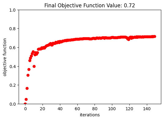
Optimization Results#
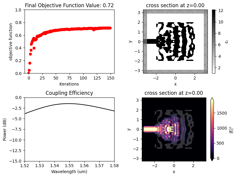
After 150 iterations, a coupling efficiency value of 0.71 (-1.48 dB) was achieved at the central wavelength.
[15]:
fig, ax = plt.subplots(1, 1, figsize=(6, 4))
ax.plot(obj_vals, "ro")
ax.set_xlabel("iterations")
ax.set_ylabel("objective function")
ax.set_ylim(0, 1)
ax.set_title(f"Final Objective Function Value: {obj_vals[-1]:.2f}")
plt.show()
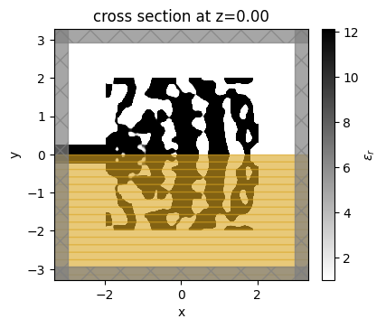
The final grating coupler structure is well binarized, with mostly black (eps_max) and white (eps_min) regions.
[20]:
fig, ax = plt.subplots(1, figsize=(4, 4))
sim_final = make_adjoint_sim(final_par, beta=final_beta, unfold=True)
sim_final = sim_final.to_simulation()[0]
sim_final.plot_eps(z=0, source_alpha=0, monitor_alpha=0, ax=ax)
plt.show()
Once the inverse design is complete, we can visualize the field distributions and the wavelength dependent coupling efficiency.
[17]:
# Field monitors to visualize the final fields.
field_xy = td.FieldMonitor(
    size=(td.inf, td.inf, 0),
    freqs=[freq],
    name="field_xy",
)

field_xz = td.FieldMonitor(
    size=(td.inf, 0, td.inf),
    freqs=[freq],
    name="field_xz",
)

# Monitor to compute the grating coupler efficiency.
gc_efficiency = td.ModeMonitor(
    center=[mon_pos_x, 0, 0],
    size=[0, mon_w, mon_h],
    freqs=freqs,
    mode_spec=mode_spec,
    name="gc_efficiency",
)

sim_final = sim_final.copy(update=dict(monitors=(field_xy, field_xz, gc_efficiency)))
sim_data_final = web.run(sim_final, task_name="inv_des_final")
           View task using web UI at                                                                  webapi.py:189
           'https://tidy3d.simulation.cloud/workbench?taskId=fdve-4d076c97-fb0c-49c2-933e-ef54b373526
           5v1'.
[18]:
mode_amps = sim_data_final["gc_efficiency"]
coeffs_f = mode_amps.amps.sel(direction="-")
power_0 = np.abs(coeffs_f.sel(mode_index=0)) ** 2
power_0_db = 10 * np.log10(power_0)

sim_plot = sim_final.updated_copy(symmetry=(0, 0, 0), monitors=(field_xy, field_xz, gc_efficiency))
sim_data_plot = sim_data_final.updated_copy(simulation=sim_plot)

f, ax = plt.subplots(2, 2, figsize=(8, 6), tight_layout=True)
sim_plot.plot_eps(z=0, source_alpha=0, monitor_alpha=0, ax=ax[0, 1])
ax[1, 0].plot(wl_range, power_0_db, "-k")
ax[1, 0].set_xlabel("Wavelength (um)")
ax[1, 0].set_ylabel("Power (dB)")
ax[1, 0].set_ylim(-15, 0)
ax[1, 0].set_xlim(wl - bw / 2, wl + bw / 2)
ax[1, 0].set_title("Coupling Efficiency")
sim_data_plot.plot_field("field_xy", "E", "abs^2", z=0, ax=ax[1, 1])
ax[0, 0].plot(obj_vals, "ro")
ax[0, 0].set_xlabel("iterations")
ax[0, 0].set_ylabel("objective function")
ax[0, 0].set_ylim(0, 1)
ax[0, 0].set_title(f"Final Objective Function Value: {obj_vals[-1]:.2f}")
plt.show()