Warm-Started Alpha Sweep#
This notebook demonstrates how to run a warm-started angle of attack (alpha) sweep. In this setup, each next case is initialized from the previous alpha solution rather than from freestream. This is achieved using the fork_from argument of project.run_case(). Warm-starting can produce more accurate results especially for conditions close to separation, as RANS simulations often get stuck in topological flow phenomena. With an initial condition closer to the final result,
warm-starting reduces the formation of non-physical separation patterns during the convergence history. Each case also uses a custom stopping criterion on CL so the solver exits as soon as convergence is reached rather than always running to max_steps.
The example uses the built-in Airplane geometry with the new mesher. After all cases finish we build a pandas DataFrame of time-averaged CL and CD values taken from results.total_forces using its get_averages() helper and plot the standard aerodynamic curves: CL vs AoA, CD vs AoA and the drag polar (CL vs CD).
1. Setup and Imports#
We import flow360 for everything related to project and case management, pandas for the post-processing dataframe and matplotlib to display the plots produced by pandas.
[1]:
import flow360 as fl
from flow360.examples import Airplane

import pandas as pd
import matplotlib.pyplot as plt
2. Project Creation#
A Flow360 Project holds the geometry asset as well as every mesh and case derived from it. We initialise the project directly from the Airplane example geometry.
[2]:
Airplane.get_files()

project = fl.Project.from_geometry(
    Airplane.geometry,
    name="Warm-Started Alpha Sweep",
)

geometry = project.geometry
[22:22:10] INFO: Geometry successfully submitted:
                   type        = Geometry
                   name        = Warm-Started Alpha Sweep
                   id          = geo-37a2ec12-19c3-4cee-b210-e473c6f616d2
                   status      = uploaded
                   project id  = prj-9ea5207f-0689-4f81-a46d-dae5f6a463f2
INFO: Waiting for geometry to be processed.
3. Meshing Parameters#
Showcasing meshing is not a goal of this tutorial, so we keep the configuration minimal:
a first boundary-layer cell thickness and a single
surface_max_edge_lengthinMeshingDefaults,a single
AutomatedFarfieldvolume zone that generates the outer farfield for us.
The new mesher is selected later on by passing use_beta_mesher=True to project.run_case().
[3]:
with fl.SI_unit_system:
    far_field_zone = fl.AutomatedFarfield()

    meshing_params = fl.MeshingParams(
        defaults=fl.MeshingDefaults(
            boundary_layer_first_layer_thickness=0.01 * fl.u.mm,
            surface_max_edge_length=0.2,
        ),
        volume_zones=[far_field_zone],
    )
[22:22:39] INFO: using: SI unit system for unit inference.
4. Simulation Parameters#
We build one SimulationParams object that will be reused for every case in the sweep. The only field we will modify between runs is operating_condition.alpha, which the loop below overwrites on each iteration.
To let the solver finish as soon as each case has settled, we attach a RunControl with a StoppingCriterion that watches CL: once the coefficient stays within a tolerance of 0.05 over a window of 200 pseudo-steps the run is terminated, even if max_steps has not been reached. A matching ForceOutput on the airplane walls exposes CL as a monitored output so the stopping criterion has a field to watch. The residual tolerances are loosened so that the force convergence
is the main condition for stopping the simulation (all criteria, including the solver tolerances must be met for the case to stop).
Note: A
CLtolerance of0.05is deliberately generous and is used here only for demonstration purposes so the cases finish quickly. For production runs you would typically pick a much tighter value matched to the accuracy you actually need.
[4]:
with fl.SI_unit_system:
    walls =fl.Wall(surfaces=[geometry["*"]])
    cl_output = fl.ForceOutput(
        output_fields=["CL"],
        models=[walls]
    )
    params = fl.SimulationParams(
        meshing=meshing_params,
        reference_geometry=fl.ReferenceGeometry(),
        operating_condition=fl.AerospaceCondition(
            velocity_magnitude=100,
            alpha=0 * fl.u.deg,
        ),
        time_stepping=fl.Steady(max_steps=4000),
        models=[
            walls,
            fl.Freestream(surfaces=[far_field_zone.farfield]),
            fl.Fluid(
                navier_stokes_solver=fl.NavierStokesSolver(
                    absolute_tolerance=1e-5
                ),
                turbulence_model_solver=fl.SpalartAllmaras(
                    absolute_tolerance=1e-5
                )
            )
        ],
        outputs=[cl_output],
        run_control=fl.RunControl(
            stopping_criteria=[
                fl.StoppingCriterion(
                    monitor_field="CL",
                    monitor_output=cl_output,
                    tolerance=0.05,
                    tolerance_window_size=200
                )
            ]
        )
    )
INFO: using: SI unit system for unit inference.
5. Running the Sweep#
We iterate through the list of alphas, updating params.operating_condition.alpha in place on every iteration and submitting a case via project.run_case(). The very first case is a regular cold-start run (no fork_from); for every subsequent alpha we pass fork_from=previous_case, which tells the platform to initialise the flow field from the previous alpha’s final solution instead of from uniform freestream.
We do not need to wait for each case to finish before submitting the next: Flow360 will schedule the forked cases on the cloud and start each of them as soon as its parent has produced a restart file. This lets us submit the whole sweep in one pass and then wait once at the end.
[5]:
alphas = [-4, 0, 4, 8, 12] * fl.u.deg

case_list = []
previous_case = None

for alpha_angle in alphas:
    params.operating_condition.alpha = alpha_angle

    if alpha_angle == alphas[0]:
        # First case: cold-start from uniform freestream.
        case = project.run_case(
            params=params,
            name=f"alpha_{alpha_angle.value}",
            use_beta_mesher=True,
        )
    else:
        # Subsequent cases: warm-start by forking from the previous alpha.
        case = project.run_case(
            params=params,
            name=f"alpha_{alpha_angle.value}",
            fork_from=previous_case,
            use_beta_mesher=True,
        )

    previous_case = case

    print(f"Submitted {case.name} (id: {case.id})")
    case_list.append((alpha_angle, case))

print("Waiting for all cases to finish...")
for _, case in case_list:
    case.wait()
print("All cases completed.")
[22:22:40] INFO: Selecting beta/in-house mesher for possible meshing tasks.
[22:22:43] INFO: Successfully submitted:
                   type        = Case
                   name        = alpha_-4
                   id          = case-cae6ebfa-19de-429c-86e0-544fe70dd03c
                   status      = pending
                   project id  = prj-9ea5207f-0689-4f81-a46d-dae5f6a463f2
Submitted alpha_-4 (id: case-cae6ebfa-19de-429c-86e0-544fe70dd03c)
[22:22:44] INFO: Selecting beta/in-house mesher for possible meshing tasks.
[22:22:46] INFO: Successfully submitted:
                   type        = Case
                   name        = alpha_0
                   id          = case-fd96b8ec-90f0-492a-a012-63127281cdc8
                   status      = pending
                   project id  = prj-9ea5207f-0689-4f81-a46d-dae5f6a463f2
Submitted alpha_0 (id: case-fd96b8ec-90f0-492a-a012-63127281cdc8)
[22:22:47] INFO: Selecting beta/in-house mesher for possible meshing tasks.
[22:22:49] INFO: Successfully submitted:
                   type        = Case
                   name        = alpha_4
                   id          = case-4dba1cb9-0c31-4c05-a976-616bc0be1bb0
                   status      = pending
                   project id  = prj-9ea5207f-0689-4f81-a46d-dae5f6a463f2
Submitted alpha_4 (id: case-4dba1cb9-0c31-4c05-a976-616bc0be1bb0)
[22:22:50] INFO: Selecting beta/in-house mesher for possible meshing tasks.
[22:22:52] INFO: Successfully submitted:
                   type        = Case
                   name        = alpha_8
                   id          = case-36c5179c-4c25-4f82-8dfa-aa8c42b0bb71
                   status      = pending
                   project id  = prj-9ea5207f-0689-4f81-a46d-dae5f6a463f2
Submitted alpha_8 (id: case-36c5179c-4c25-4f82-8dfa-aa8c42b0bb71)
[22:22:53] INFO: Selecting beta/in-house mesher for possible meshing tasks.
[22:22:55] INFO: Successfully submitted:
                   type        = Case
                   name        = alpha_12
                   id          = case-af2bd93e-4855-447c-abfe-9dab43855d9e
                   status      = pending
                   project id  = prj-9ea5207f-0689-4f81-a46d-dae5f6a463f2
Submitted alpha_12 (id: case-af2bd93e-4855-447c-abfe-9dab43855d9e)
Waiting for all cases to finish...
All cases completed.
6. Post-Processing#
With the sweep finished we collect averaged total force coefficients from each case. case.results.total_forces exposes a get_averages(fraction) helper that returns the mean of the last fraction of pseudo-steps as a pandas Series, so we can index directly into it to obtain the converged CL and CD.
[6]:
records = []
for alpha_angle, case in case_list:
    averages = case.results.total_forces.get_averages(0.1)
    records.append(
        {
            "alpha_deg": float(alpha_angle.to("deg").value),
            "CL": averages["CL"],
            "CD": averages["CD"],
        }
    )

sweep = pd.DataFrame(records).sort_values("alpha_deg").reset_index(drop=True)
print(sweep)
[23:00:09] INFO: Saved to C:\Users\Piotr\AppData\Local\Temp\tmpz_p_3h1s\ccb1d2ec-769a-415f-963e-ab4107915615.csv
[23:00:12] INFO: Saved to C:\Users\Piotr\AppData\Local\Temp\tmpz_p_3h1s\55abf9de-19a6-4fea-affe-4ef66a558c3d.csv
[23:00:14] INFO: Saved to C:\Users\Piotr\AppData\Local\Temp\tmpz_p_3h1s\d1c7d713-bc47-40cc-8b05-45d14f6f9dd2.csv
[23:00:16] INFO: Saved to C:\Users\Piotr\AppData\Local\Temp\tmpz_p_3h1s\ca7c651e-efdf-4b34-ad14-61f8fa17a772.csv
[23:00:19] INFO: Saved to C:\Users\Piotr\AppData\Local\Temp\tmpz_p_3h1s\9b311da0-e62c-42ca-b8f9-e0d6f0069fb0.csv
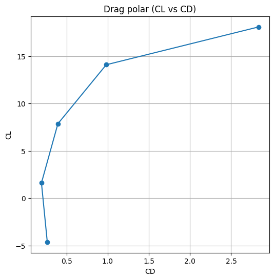
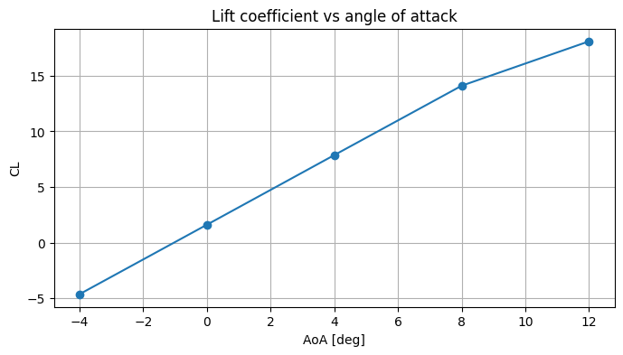
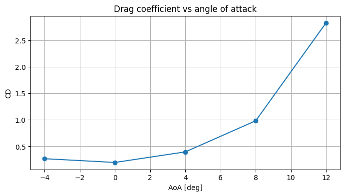
   alpha_deg         CL        CD
0       -4.0  -4.623297  0.266586
1        0.0   1.617527  0.195803
2        4.0   7.870213  0.395486
3        8.0  14.101717  0.982705
4       12.0  18.091709  2.830544
CL vs AOA, CD vs AOA and the drag polar#
Pandas’ built-in DataFrame.plot() is convenient for quick engineering plots. We produce three panels: the lift curve, the drag curve and the drag polar.
[7]:
ax = sweep.plot(
    x="alpha_deg",
    y="CL",
    marker="o",
    legend=False,
    xlabel="AoA [deg]",
    ylabel="CL",
    title="Lift coefficient vs angle of attack",
    figsize=(8, 4),
)
ax.grid(True)
plt.show()
[8]:
ax = sweep.plot(
    x="alpha_deg",
    y="CD",
    marker="o",
    legend=False,
    xlabel="AoA [deg]",
    ylabel="CD",
    title="Drag coefficient vs angle of attack",
    figsize=(8, 4),
)
ax.grid(True)
plt.show()
[9]:
ax = sweep.plot(
    x="CD",
    y="CL",
    marker="o",
    legend=False,
    xlabel="CD",
    ylabel="CL",
    title="Drag polar (CL vs CD)",
    figsize=(6, 6),
)
ax.grid(True)
plt.show()