User Defined Dynamics#
In Flow360, users are able to specify arbitrary dynamics. This section provides an example for a Proportional-Integral (PI) controller and an example for Aero-Structural Interaction (ASI).
PI Controller for Angle of Attack to Control Lift Coefficient#
In this example, we add a controller to the om6Wing case study. Based on the entries of the configuration file in this case study, the resulting value of the lift coefficient, CL, obtained from the simulation is ~0.26. Our objective is to add a controller to this case study such that for a given target value of CL (e.g., 0.4), the required angle of attack, alphaAngle , is estimated. To this end, a PI controller is defined under userDefinedDynamics in the configuration file as:
"userDefinedDynamics": [
    {
        "dynamicsName": "alphaController",
        "inputVars": [
            "CL"
        ],
        "constants": {
            "CLTarget": 0.4,
            "Kp": 0.2,
            "Ki": 0.002
        },
        "outputVars": {
            "alphaAngle": "if (pseudoStep > 500) state[0]; else alphaAngle;"
        },
        "stateVarsInitialValue": [
            "alphaAngle",
            "0.0"
        ],
        "updateLaw": [
            "if (pseudoStep > 500) state[0] + Kp * (CLTarget - CL) + Ki * state[1]; else state[0];",
            "if (pseudoStep > 500) state[1] + (CLTarget - CL); else state[1];"
        ],
        "inputBoundaryPatches": [
            "1"
        ]
    }
]
More details for some of the parameters are explained below:
dynamicsName: This is a name given by the user for the dynamics. The results of user-defined dynamics are saved to “udd_dynamicsName_v2.csv”.
constants: This includes a list of all the constants related to this UDD. These constants will be used in the equations for
updateLawandoutputVars. In the above-mentioned example,CLTarget,Kp, andKiare the target value of the lift coefficient, the proportional gain of the controller, and the integral gain of the controller, respectively.outputVars: Each
outputVarsconsists of the variable name and the relations between the variable and the state variables. For this example, we set the output variable equal to the angle of attack calculated by the controller after the first 500 pseudoSteps (i.e.,state[0]).stateVarsInitialValue: There are two state variables for this controller. The first one,
state[0], is the angle of attack computed by the controller, and the second one,state[1], is the summation of error(CLTarget - CL)over iterations. The initial values ofstate[0]andstate[1]are set toalphaAngleand0, respectively.
The equation for the control system can be thus written as:
where the superscript \(n\) denotes pseudo step, alphaAngle (\(\alpha\)) is state[0] and the integral of error (\(e\)) is state[1].
updateLaw: The expressions for the state variables are specified here. The first and the second expressions correspond to equations for
state[0]andstate[1], respectively. The conditional statement forces the controller to not be run for the first 500 pseudoSteps. This ensures that the flow field is established before the controller is initialized.inputBoundaryPatches: The related boundary conditions for the inputs of the user-defined dynamics are specified here. In this example, the noSlipWall boundary conditions are where
CLis calculated. As seen in the configuration file, the boundary name for the No-Slip boundary condition is"1".
The following figure shows the values of lift coefficient, CL, and angle of attack, alphaAngle, versus the steps, pseudoStep. As specified in the configuration file, the initial value of angle of attack is 3.06. With the specified user-defined dynamics, alphaAngle is adjusted to a final value of 4.61 so that CL = 0.4 is achieved.
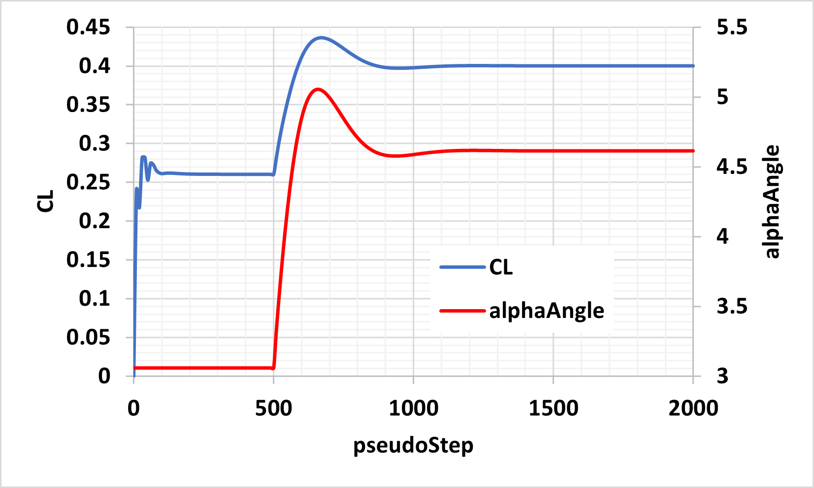
Fig. 243 Results of alphaController for om6Wing case study.#
Dynamic Grid Rotation using Structural Aerodynamic Load#
In this example, we present an illustrative case where a flat plate rotates while being subjected to a rotational spring moment and damper as well as aerodynamic loads.
As you can see below, the flate plate mesh consists of two zones separated by a circular sliding interface. The inner zone will rotate while the outer zone remains stationary. This is the same mesh topology as what is used for rotating propeller simulations.
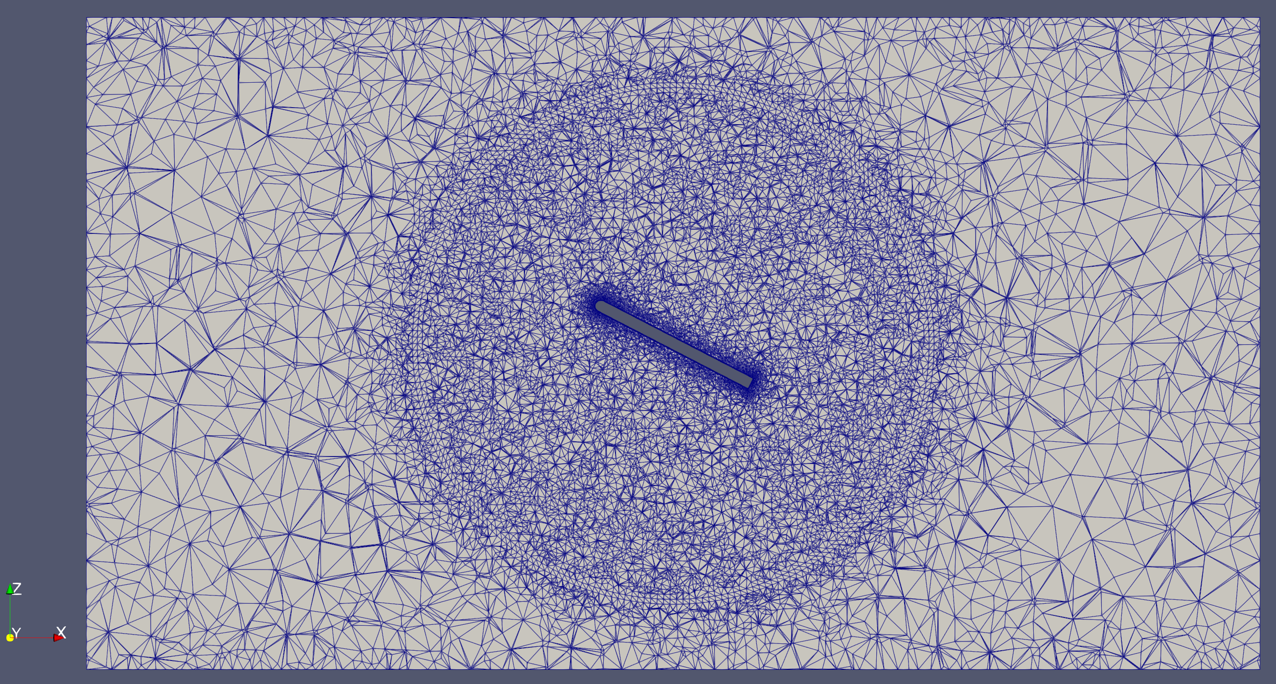
Fig. 244 Mesh of flat plate showing sliding interface for rotation.#
Below is a video showing the flutter motion of the plate.
Fig. 245 Flutter motion of the plate under aerodynamic and structural forces.#
The userDefinedDynamics and slidingInterfaces section of the case JSON is presented below:
 1{
 2    "slidingInterfaces": [
 3        {
 4            "stationaryPatches": [
 5                "farFieldBlock/rotIntf"
 6            ],
 7            "rotatingPatches": [
 8                "plateBlock/rotIntf"
 9            ],
10            "axisOfRotation": [
11                0,
12                1,
13                0
14            ],
15            "centerOfRotation": [
16                0,
17                0,
18                0
19            ],
20            "volumeName": "plateBlock",
21            "theta": [
22                "0",
23                "0",
24                "0"
25            ]
26        }
27    ],
28    "userDefinedDynamics": [
29        {
30            "dynamicsName": "dynamicTheta",
31            "inputVars": [
32                "momentY"
33            ],
34            "constants": {
35                "I": 0.443768309310345,
36                "zeta": 4.0,
37                "K": 0.0161227107,
38                "omegaN": 0.190607889,
39                "theta0": 0.0872664626
40            },
41            "outputVars": {
42                "omegaDot": "state[0];",
43                "omega": "state[1];",
44                "theta": "state[2];"
45            },
46            "stateVarsInitialValue": [
47                "-1.82621384e-02",
48                "0.0",
49                "1.39626340e-01"
50            ],
51            "updateLaw": [
52                "if (pseudoStep == 0) (momentY - K * ( state[2] - theta0 ) - 2 * zeta * omegaN * I *state[1] ) / I; else state[0];",
53                "if (pseudoStep == 0) state[1] + state[0] * timeStepSize; else state[1];",
54                "if (pseudoStep == 0) state[2] + state[1] * timeStepSize; else state[2];"
55            ],
56            "inputBoundaryPatches": [
57                "plateBlock/noSlipWall"
58            ],
59            "outputTargetName": "plateBlock"
60        }
61    ]
62}
For this case the dynamics of the plate are:
which corresponds to the three updateLaw arguments in the above JSON input file. The symbols are defined in the table below.
Symbol |
Description |
|---|---|
\(\theta\) |
Rotation angle of the plate in radians. |
\(\omega\) |
Rotation velocity of the plate in radians. |
\(\dot{\omega}\) |
Rotation acceleration of the plate in radians. |
\(\tau_y\) |
Aerodynamic moment exerted on the plate. |
\(K\) |
Stiffness of the spring attached to the plate at the structural support. |
\(\zeta\) |
Structural damping ratio. |
\(\omega_N\) |
Structural natural angular frequency. |
\(I\) |
Structural moment of inertia. |
In the inputVars, the momentY is the y-component of the rotational moment imposed by the aerodynamic loading. The moment is calculated relative to the momentCenter on "plateBlock/noSlipWall".
The name of rotating volume zone that we want to control is plateBlock and thus the "outputTargetName" is set to plateBlock. The first, second and third state variable correspond to \(\dot{\omega}\), \(\omega\), and \(\theta\), respectively.